Generate vascular trees in uniform and locally refined domains

These examples run the C++ vascular_network application before any transient simulation. They use synthetic SI data, not a calibrated organ model. The vascular generation guide describes the library, completion of imported networks, distributed growth, physical laws and failure reports.

The four domains start with one uniform refinement. The adaptive cube then refines towards the edge parallel to \(x\) at \(y=z=1\), at distances \(0.45L,0.225L,0.1125L\) for cube side \(L\). The adaptive sphere refines towards its center at distances \(R/2,R/4,R/8\) for sphere radius \(R\). These are ordinary deal.II refinement passes, completed before generation. Growth does not adapt the mesh.

Parameter	Value
Cube origin and side	\((0,0,0)\); \(L=1\ \mathrm{m}\)
Sphere center and radius	\((0.5,0.5,0.5)\ \mathrm{m}\); \(R=0.5\ \mathrm{m}\)
Arterial seed	Cube: \((0.05,0.25,0.25)\ \mathrm{m}\); sphere: \((0.2,0.5,0.5)\ \mathrm{m}\)
Initial direction and fixed seed radius	Positive \(x\); \(0.003\ \mathrm{m}\)
Length policy and seed coefficient	local mesh size; \(1\)
Minimum normalized vessel length; clearance	\(0.1\); \(0\)
Dynamic viscosity	\(0.004\ \mathrm{Pa\,s}\)
Total new-tissue reference flow	\(2\times10^{-9}\ \mathrm{m^3/s}\)
Arterial inlet pressure	\(12000\ \mathrm{Pa}\)
Murray exponents; tissue density; spatial weight	\(3\); \(1\); \(1\)
Sampling seed and terminal count	\(23\); one per global active background cell
Density mesh exponent \(\beta\)	\(3\) on every background
Maximum service distance	One local cell diameter at each tissue quadrature point
Terminal-count calibration	Disabled: volume and coverage targets are zero
Numerical interval target and desired range	\(h\); \(0.5h\)–\(2h\)

Each cube pair and sphere pair keeps its physical controls unchanged. Refining the background changes terminal count and geometric scales automatically. Territorial demand integrates the constant density over the physical tissue; adding terminals redistributes that integral and the same total flow. These single-seed figures illustrate the ordinary configuration. The mesh-refinement study compares three uniform/local resolutions across several seeds, without imposing geometrical identity or statistical-equivalence thresholds. Separate calibration tests retain the volume/coverage target checks.

The source configurations are uniform cube, edge cube, uniform sphere and central sphere. CMake generates their runtime .prm files below the build tree. All effective parameters record every native parameter, including defaults. Only the run-directory prefix is replaced by <run> in that published record.

Networks and backgrounds

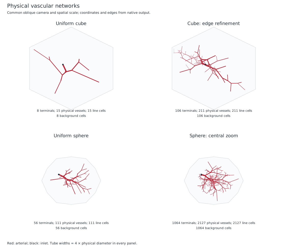
The camera, spatial scale and vessel-width scale are common to all four panels. Tube widths are four times physical diameter to make the radii legible; the stored radii are unchanged. Black dots mark the explicit inlet ports. The gray outline is the convex hull of projected native mesh vertices, not a generated replacement mesh.

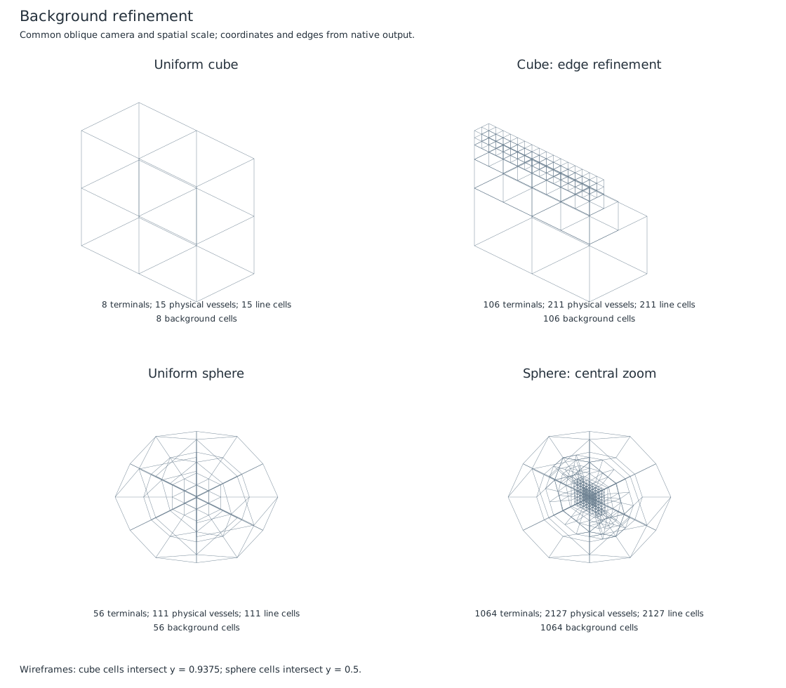
The cube wireframes show cells intersecting \(y=0.9375\), close to the refined edge. Sphere wireframes use \(y=0.5\). Both include cells on either side of the selected plane. The central sphere panel resolves the nested refinement regions. First-order mappings approximate the spherical boundary. Reported volume fractions use each actual native background volume, not \(4\pi R^3/3\).

Physical terminal density and numerical cell length

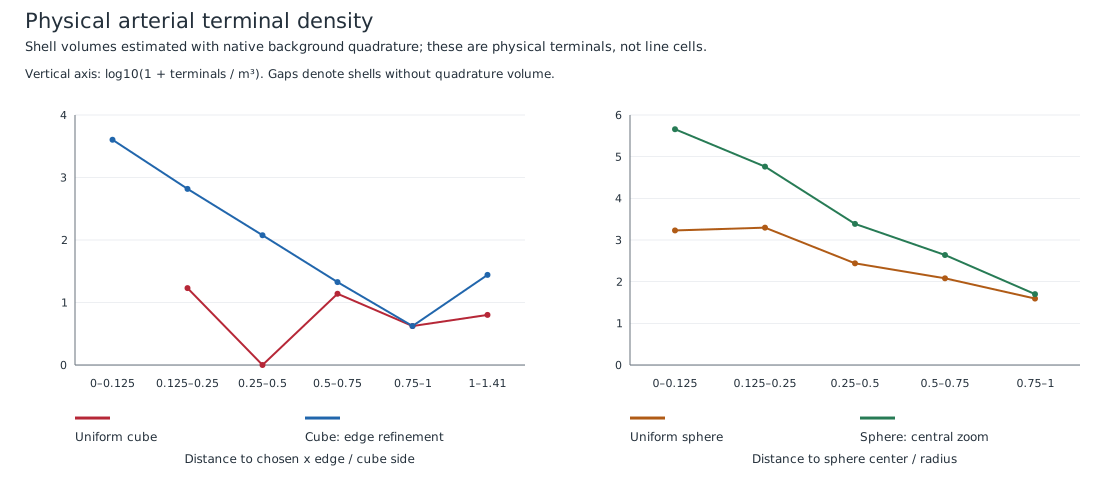
The denominator is the sum of native background QGauss(2) physical weights in each distance bin. The numerator counts owned physical arterial tissue terminals. This is a quadrature estimate of shell volume. A shell with no quadrature volume has no plotted density. The logarithmic vertical coordinate is \(\log_{10}(1+\rho_T)\), with density in terminals per cubic metre.

All cases use \(\beta=3\), giving comparable proposal weight per cell when the spatial weight is one. Smaller cells therefore receive more proposals per unit physical volume. Geometric acceptance can change that distribution. These single-seed examples do not establish statistical quality across partitions or seeds.

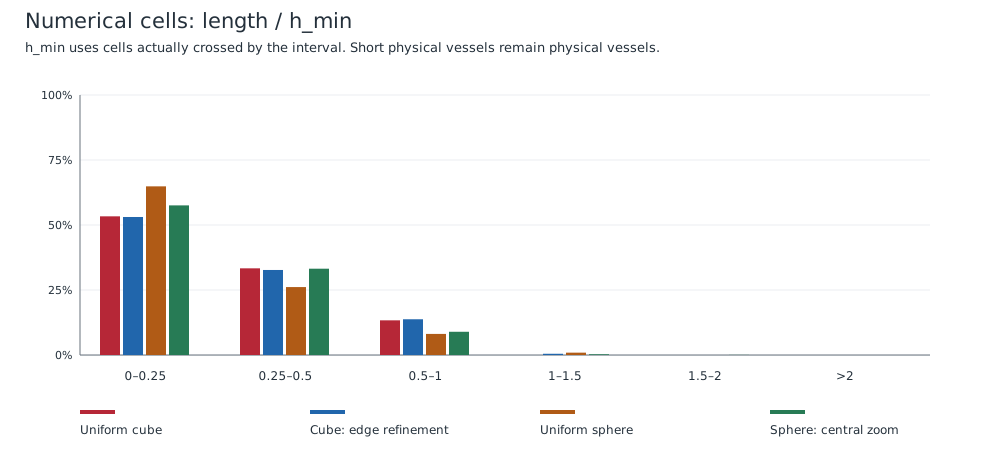
Each histogram counts numerical intervals. Its denominator \(h_{\min}\) comes from background cells actually crossed by the interval. Short physical branches and crossing fragments can fall below the desired \(0.5h\) bound; the native interval table records short-cell exceptions. Subdivision preserves each physical vessel’s integrated volume and Poiseuille resistance and creates no new bifurcation.

Physical volume and geometric coverage

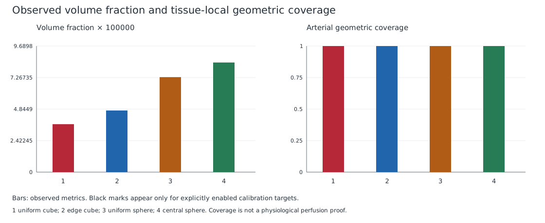
The bars report observed volume and coverage, with calibration disabled. A nearest-territory assignment contributes integrated demand even where the service-distance criterion reports uncovered tissue. Coverage uses the tissue point’s local cell diameter and remains separate from physiological perfusion.

Measured run summary records counts, volume fraction, coverage and calibration results. The full owned tables, archives and meshes remain in the build tree.

Arterial and venous common territories

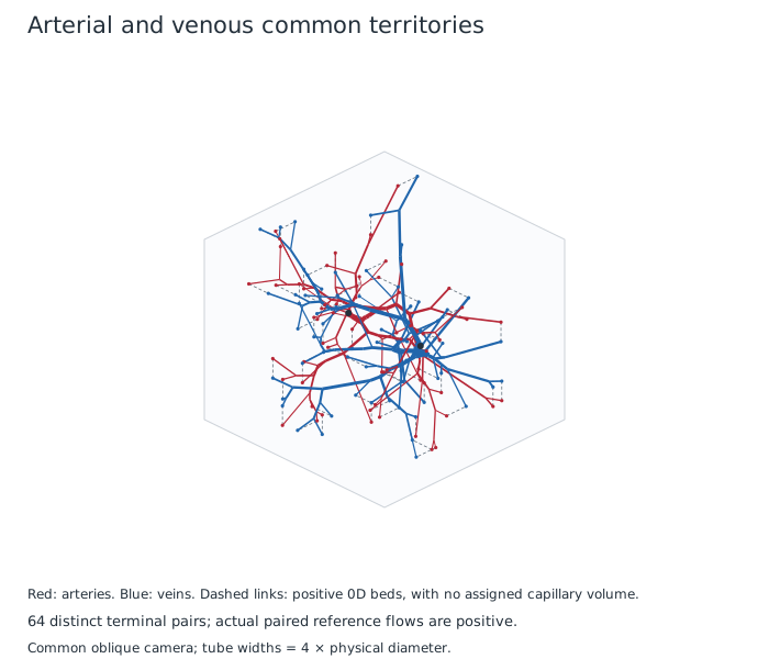
The arterial–venous configuration adds a venous outlet at \((0.95,0.75,0.75)\ \mathrm{m}\) with fixed radius \(0.004\ \mathrm{m}\) and pressure \(4000\ \mathrm{Pa}\). This example uses two uniform background refinements. Terminal partners are \(0.25H\) apart, with \(H\) evaluated once at their common territory centre. A positive resistance for each bed is derived from the explicit pressure data and integrated demand flow, then checked in the actual paired reference solve. Calibration remains disabled.

Dashed links identify the common territories. They are 0D resistive connections, not capillary segments with an implicit volume. Veins grow from the outlet towards the tissue; their reference flow has the opposite orientation. These reference results precede any transient haemodynamic simulation.

Rediscretize the same physical graph

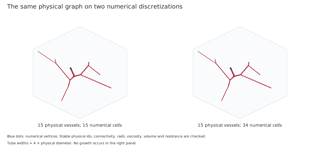
The load-only configuration reloads the uniform cube archive without growth. It uses four uniform background refinements and the same target interval length \(h\), with desired range \(0.5h\)–\(2h\). The pipeline checks identical physical ids, connectivity, geometry, radii and viscosity, and independently integrates every interval to check preservation of physical volume and resistance. Only numerical cells and vertices change. Normalized length/radius diagnostics and tissue-local coverage also change with the new background scale; the stored physical graph stays the same.

Reproduce and check the published figures

Build the standalone target using an installed deal.II, with MetricFlowX disabled if desired:

cmake -S . -B /tmp/immersx-vascular-build -DCMAKE_BUILD_TYPE=Release \
  -DCMAKE_DISABLE_FIND_PACKAGE_MetricFlowX=ON
cmake --build /tmp/immersx-vascular-build --target vascular_network -j
python3 scripts/run_vascular_examples.py \
  --executable /tmp/immersx-vascular-build/vascular_network \
  --parameters /tmp/immersx-vascular-build/data/vascularization \
  --output /tmp/immersx-vascular-build/vascular-examples-1
python3 scripts/update_vascular_figures.py \
  /tmp/immersx-vascular-build/vascular-examples-1 --check

The output directory must be new. The runner launches every executable from an unrelated working directory and retains logs, effective parameters, distributed archives and tables below that run directory. The Python scripts perform no vascular growth. They validate and plot owned C++ output with the standard library, without a rendering dependency.

To refresh selected assets after reviewing a fresh run, omit --check. To test reproducibility, run the generator again into a second new directory and check it against the published assets. The manifest records the fixed projection, diameter exaggeration and asset hashes. Equality applies to the recorded seed, parameters, process count and numerical environment. Different MPI partitions may produce different valid geometry and are not compared byte for byte.

CTest also runs the six examples through ImmersX.Application.vascular_network.IllustratedExamples (with _debug in the executable name for Debug). It retains a unique build-tree directory for each run. Pass --ranks 2 --mpiexec /path/to/mpirun to the runner for an MPI run; its invariant checks apply to the combined owned records. MPI scaling benchmarks are separate from these small illustrated cases.

Generate before the coupled transient solve

With a compatible MetricFlowX package installed, metric_flow_x_elastodynamics can generate a validated internal network on the solid’s final background before distributing native flow DoFs and constructing the existing wall coupling. The generator itself still builds without MetricFlowX.

The small coupled configuration uses a unit cube with 64 solid cells and a four-terminal arterial tree. Its seed, viscosity and reference-flow data match the synthetic values above; the terminal count is fixed, with no volume calibration or minimum-coverage target. Native Square root walls use Young modulus 5e5 Pa, wall thickness 0.0003 m, and reference pressure 125 Pa. Each tissue outlet uses native R1=0, R2=1e8 Pa s/m^3, C=0 and the same 125 Pa reservoir pressure. The equal nonzero reference and outlet pressures balance at rest; the pressure reference is assigned once to native p_d, with native p0=0.

The inherited time-dependent inflow is \(Q(t)=5\times10^{-8}(1-\cos(100\pi t))\ \mathrm{m^3/s}\). Both \(Q(0)\) and \(Q'(0)\) vanish, matching the initially resting solid; the inflow is nonzero at subsequent times. This transient forcing is distinct from the 2e-9 m^3/s resistive design flow used during generation. IDA advances from zero to 0.002 s, with flow, solid and pressure-jump output at 0, 0.001 and 0.002 s.

Configure both packages against the same deal.II installation and linear algebra backend. This checkout selects Trilinos, so configure the native package with -DMETRIC_FLOW_X_BACKEND=Trilinos. For example:

cmake -S . -B build-coupled -DCMAKE_BUILD_TYPE=DebugRelease \
  -DMetricFlowX_DIR=/path/to/metric-flow-x-install/lib/cmake/MetricFlowX \
  -DENABLE_GOOGLE_TESTING=ON
cmake --build build-coupled --target \
  metric_flow_x_elastodynamics metric_flow_x_elastodynamics_debug -j
ctest --test-dir build-coupled \
  -R 'application\.MetricFlowXGenerated\.' --output-on-failure

CTest creates separate parameter and output paths for each build variant and solver mode. The checks require actual accepted IDA steps, nonempty internal vessel geometry, the three output times, positive flow-state change and positive solid displacement. Available direct-solver cases include serial UMFPACK and serial/two-rank/four-rank MUMPS. An older MetricFlowX package without the native in-memory input API skips these generated-input cases.

For a new application, follow the native transfer example. It explains owner-local material callbacks, explicit terminal data, native coefficient replication, stable physical IDs and reversed venous execution orientation. Partially external imported networks remain supported by the standalone generator; adapting their multiplier space for partial wall coupling is deferred.

Measured background-refinement study

The native generator completed all 18 cases: three uniform and three edge resolutions, each with seeds 23, 24 and 25. The physical inlet, root radius, viscosity, pressure and total flow are fixed. Growth uses the ordinary mesh controls in the table above. Only background refinement and seed vary.

The ranges below span the three per-seed medians. Length is the whole-branch integral \(\int ds/H\); radius is the minimum \(r/H\) along that branch.

Background	Level	Cells and terminals	Median normalized length	Median minimum \(r/H\)
Uniform	1	8	0.184–0.275	0.00193–0.00202
Uniform	2	64	0.189–0.233	0.00196–0.00200
Uniform	3	512	0.201–0.212	0.00202–0.00203
Edge	1	22	0.219–0.245	0.00200–0.00228
Edge	2	50	0.189–0.249	0.00198–0.00233
Edge	3	106	0.221–0.232	0.00211–0.00230

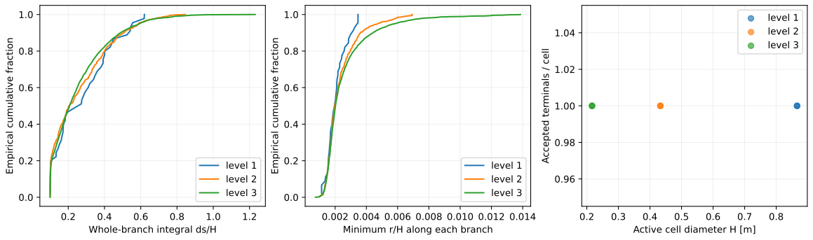
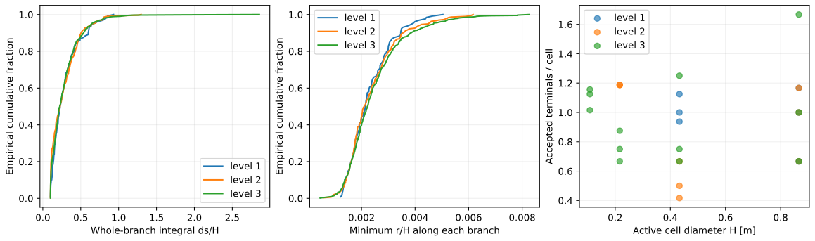
The cumulative curves pool branches across the three seeds. The right panels retain individual seed counts within each cell-diameter group. The global terminal/cell ratio is one by the count policy; these conditional counts show how geometric acceptance changes its spatial allocation. At the finest edge resolution, the 64 smallest cells contain 65, 74 and 72 terminals respectively.

Every case conserves demand per tissue volume at 1 and total flow per tissue volume at \(2\times10^{-9}\ \mathrm{s^{-1}}\), within the independent table oracle’s floating-point tolerances. All generated branches satisfy the 0.1 minimum normalized length. These observations support comparable local scales for this experiment; no equivalence threshold is imposed. The fixed physical root radius gives a growing \(r/H\) at the root under uniform refinement, so the upper radius tails need not coincide.

The per-seed summary, individual distributions and work counters, shared physical controls and source/binary manifest retain the measurements. Follow the refinement-study workflow to reproduce them. The executable, library and scripts are hashed; timings were collected alongside other validation work on separate worker cores and are not isolated performance estimates.

Integrated-demand cost checks

Two representative native Release runs completed with 1,000 and 10,000 terminals. Both use seed 23, one MPI rank, a unit cube with 512 background cells, a 0.003 m fixed root radius, 0.004 Pa s viscosity, 12000 Pa inlet pressure and total flow \(2\times10^{-9}\ \mathrm{m^3/s}\). This cost protocol uses Length scale = meter, absolute terminal counts, density exponent zero, seed length 0.15 and minimum vessel length zero. It measures the same integrated territory model as ordinary mesh-driven growth; its absolute-count controls permit these two requested sizes on the same background.

Terminals	Tissue quadrature points	Generation [s]	Peak rank RSS [KiB]
1,000	262,144	42.568	411,456
10,000	2,097,152	985.885	1,374,120

Each run passes the independent tree, demand conservation, Murray radius, physical interval, total-flow and pressure-drop checks. Initialization and finalization are excluded from the ordinary operation counts below; their time is included in the generation totals above.

Ordinary operation	1,000 terminals	10,000 terminals
Background cache constructions	0	0
Background cell visits	0	0
Materialized physical vessels	0	0
Physical vessel copy attempts	2,997	29,997
Vessel midpoint localizations	2,997	29,997
Physiology branch visits	50,116	837,906
Candidate ancestor-path visits	11,100,511	240,200,623
Tissue influence-query hits	2,730,667	30,822,458
Reassigned tissue samples	1,582,623	17,474,781
Exact vessel-pair checks	946,548	10,222,329

Ten times as many terminals take about 23.2 times the generation time in these runs. The quadrature is eight times larger. Candidate-path visits grow about 21.6 times; this counter includes ancestor traversals across optimization trials. Copies and midpoint localization remain exactly \(3(N-1)\); the zero bulk counters exclude repeated full background scans or physical-network materialization during insertion. These two sizes do not establish asymptotic scaling or a speedup against the historical point-demand model, whose physiology and proposal trajectories differ.

The executable, shared library and scripts are pinned in the experiment manifest. Per-size summary, native measurements and phase counters and worker protocol retain the evidence. No agent C++ compiler ran during these measurements; other validation and the independent incremental-growth campaign used separate cores. These are observed worker costs, with one seed per size, rather than an isolated timing study or an MPI scaling result.

Historical MPI growth baseline

These archived measurements describe the earlier point-demand generator, not the current integrated-demand implementation. They are retained as the cost baseline; the frozen source and binary identities are recorded below. Current measurements must report their own quadrature sizes and work counters.

The baseline uses three random seeds (23, 24, 25) for every process-count and size combination: 1,000 and 10,000 terminals at P=1,2,4,8 for strong scaling, and 1,000 terminals per process at P=1,8 for weak scaling. Every one of the 30 native runs passed the independent table checks described in the generation guide. The figures show medians and full observed seed ranges; they do not fit a model.

Protocol	MPI ranks	Generation time: median [min, max], seconds
strong, T=1,000	1	144.3 [143.2, 144.8]
strong, T=1,000	2	46.52 [44.08, 48.44]
strong, T=1,000	4	15.24 [15.21, 15.32]
strong, T=1,000	8	5.549 [5.466, 5.996]
strong, T=10,000	1	1.418e+04 [1.415e+04, 1.427e+04]
strong, T=10,000	2	3691 [3631, 4069]
strong, T=10,000	4	997 [994.2, 1000]
strong, T=10,000	8	283.9 [273.5, 285.4]
weak, T=1,000 per rank	1	142.4 [140.5, 145.2]
weak, T=1,000 per rank	8	227.9 [227.1, 229.2]

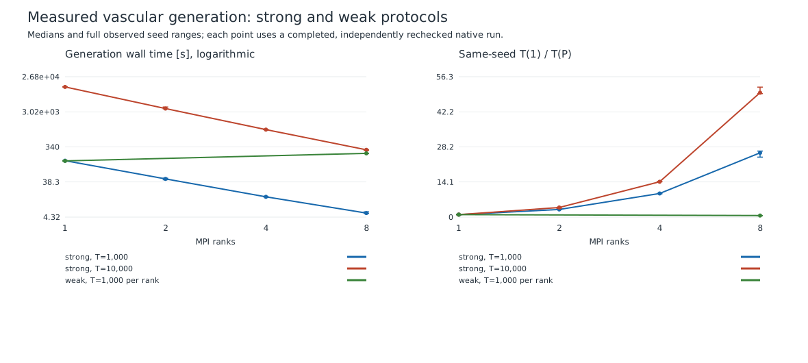
The strong protocol keeps terminal count and physical controls fixed, but changing the number of processes changes batch size, sampled geometry and the number of global physiological updates. Ratios above the process count therefore include changes in algorithmic work; they are not hardware speedups for an identical sequence of insertions. The weak protocol grows one connected tree from one real inlet as the domain and terminal count increase. It does not create independent roots to give every rank work.

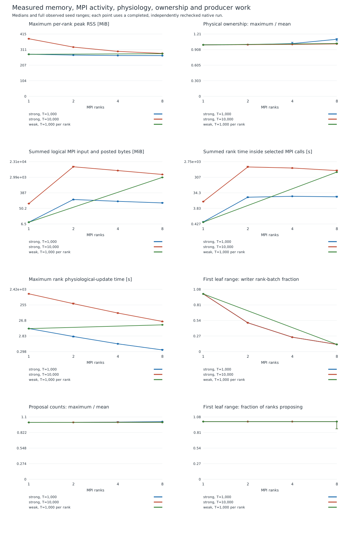
Peak RSS is the maximum per-rank high-water mark. The CSV also retains the sum of individual peaks; that sum counts shared pages repeatedly and does not measure simultaneous node memory. MPI bytes are logical posted sends plus collective input, not wire traffic. MPI seconds sum rank time inside the instrumented calls and can exceed elapsed time. The first-range writer fraction measures ownership of mutable branches across rank-batches; it does not count all CPU-active proposal producers. The separate first-range proposer fraction counts ranks with at least one proposal. Whole-growth phase times use the maximum of per-rank totals rather than a sum of range maxima.

Protocol	MPI ranks	Volume fraction: median [min, max]	Arterial coverage: median [min, max]
strong, T=1,000	1	6.905e-05 [6.847e-05, 6.96e-05]	1 [1, 1]
strong, T=1,000	2	6.846e-05 [6.806e-05, 6.853e-05]	1 [0.9998, 1]
strong, T=1,000	4	6.819e-05 [6.807e-05, 6.943e-05]	1 [1, 1]
strong, T=1,000	8	6.85e-05 [6.7e-05, 6.865e-05]	1 [1, 1]
strong, T=10,000	1	8.913e-05 [8.842e-05, 8.955e-05]	1 [1, 1]
strong, T=10,000	2	8.875e-05 [8.866e-05, 8.879e-05]	1 [1, 1]
strong, T=10,000	4	8.898e-05 [8.851e-05, 8.905e-05]	1 [1, 1]
strong, T=10,000	8	8.889e-05 [8.884e-05, 8.906e-05]	1 [1, 1]
weak, T=1,000 per rank	1	6.905e-05 [6.847e-05, 6.96e-05]	1 [1, 1]
weak, T=1,000 per rank	8	8.684e-05 [8.665e-05, 8.708e-05]	1 [1, 1]

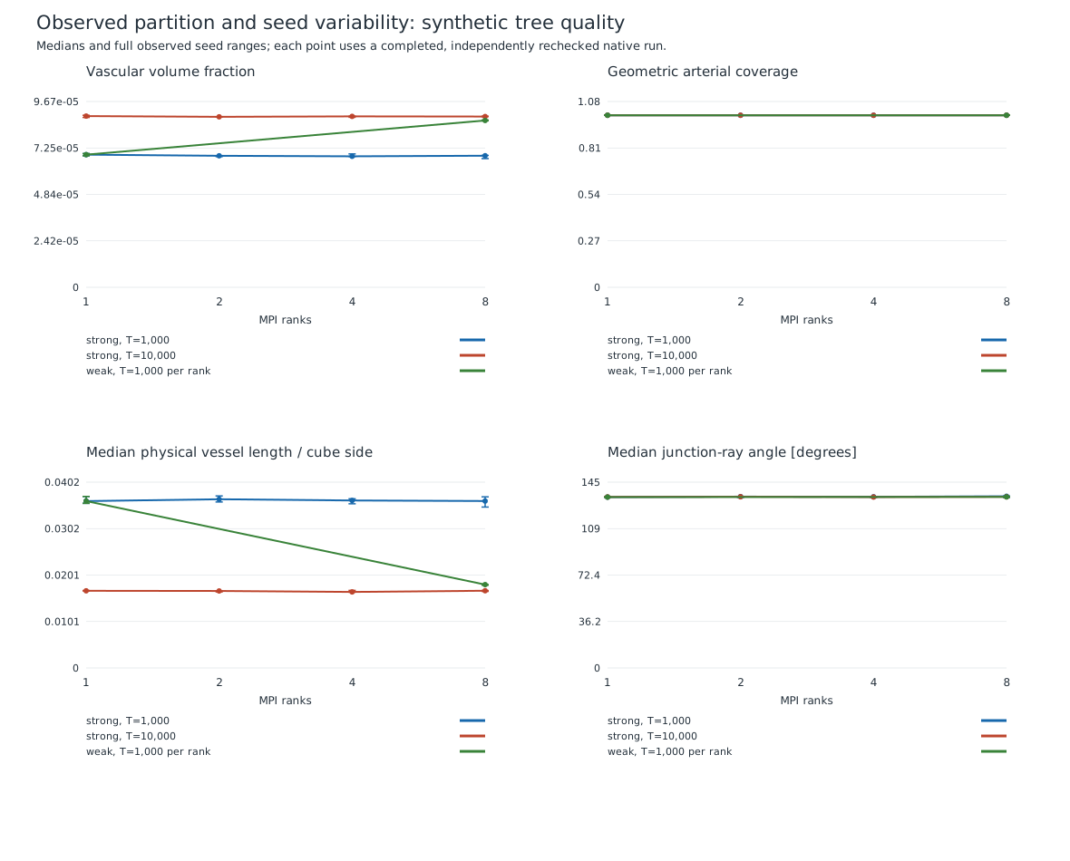
All runs satisfy the same topology, Murray, wall-containment, junction-angle, flow and subdivision checks. The plotted distributions describe the observed seed and partition variability. Three seeds do not establish statistical equivalence, and these synthetic geometric measurements do not establish physiological perfusion. The benchmarks prescribe terminal counts; they do not calibrate a target volume fraction or enforce a minimum coverage.

The smallest recorded reference area across these trees is 6.0915206e-08 m². The native transfer requires an area strictly above 1e-10 m² and rejects smaller physical radii instead of clipping them. This comparison uses the generated radii; the generation benchmarks do not advance the transient flow solver.

Per-seed measurements include radius and terminal-distance quantiles in addition to the plotted metrics, plus per-rank sample, proposal and accepted-insertion counts and their maximum-to-mean ratios. The manifest records the source and binary identities, input hashes and asset hashes.

Recorded environment

The recorded runs use an Intel Xeon E5-2650 v4 host, GCC 11.4.0, deal.II 9.8.0 and Open MPI 5.0.10. They use the Release targets of a DebugRelease configuration with one OpenMP and one OpenBLAS thread per process. Effective compilation includes -DNDEBUG -O2 -fopenmp, -fopenmp-simd -march=znver3 -mtune=znver3; the architecture flags come from the installed SDK and are recorded as used, despite the Intel host. The frozen benchmark executables and library use the gold linker. These are recorded local build conditions, not required project flags.

MPI processes use --bind-to core --report-bindings. Other local builds, functional tests and documentation work used separate cores where possible, while the host also served unrelated work. Memory bandwidth, cache and storage remained shared. Treat the timings as shared-host measurements rather than isolated machine performance.

The frozen generator source is 76bb381187285e57bdc281a09f2bdd4c09a70703. The executable SHA-256 is d4a70de019707637c76897b44dd33723a5cc3a1805793abc784467096f8a06ca and the library SHA-256 is 559e03f47fe7a6e041f40bf6d134a133b8f2c2b3b5b28965dd70e0c29b9eb082. These files were copied before the experiments and were not rebuilt between cases.

Reproduce the historical baseline

The archived manifests retain the exact inputs, commands, source identity and binary hashes. Reproducing these figures requires the corresponding archived source and scripts. Do not rerun the old multi-hour campaign merely to establish the baseline. The current benchmark runner validates integrated territory weights and records the new execution counters; use the current measurement workflow for that implementation. Keep the two physical-demand protocols separate when comparing timings and quality.