Vascularize a liver from a surface and two 1D trees

This tutorial starts with a closed liver surface and two rooted 1D vessel meshes. Domain<3,3> meshes the enclosed tissue with the Gmsh API. The liver_vascular application then extends the supplied arterial and venous leaves toward common tissue territories. The supplied nodes, vessels and radii remain fixed during growth.

        flowchart LR
  S[Closed liver surface] --> M[Gmsh volume mesh]
  A[Arterial 1D tree] --> G[Paired vascular growth]
  V[Venous 1D tree] --> G
  M --> G
  G --> O[Vascularized tissue and physical archive]
    

The worked example uses 3D-IRCADb-1, case 12. The IRCAD download contains organ and vessel surface meshes, rather than ready-made centerlines. A preparation script extracts approximate centerlines and writes ordinary 1D VTK meshes. If you already have suitable 1D meshes, start at Describe the input trees.

This is a geometric growth example. The pressures, flow and extension settings below are illustrative, not a patient calibration. The example uses hepatic arterial supply and a retained hepatic venous tree. The published two-network run below omits portal inflow. The three-network extension adds that role through a common microvascular compartment; these examples do not establish physiological liver perfusion.

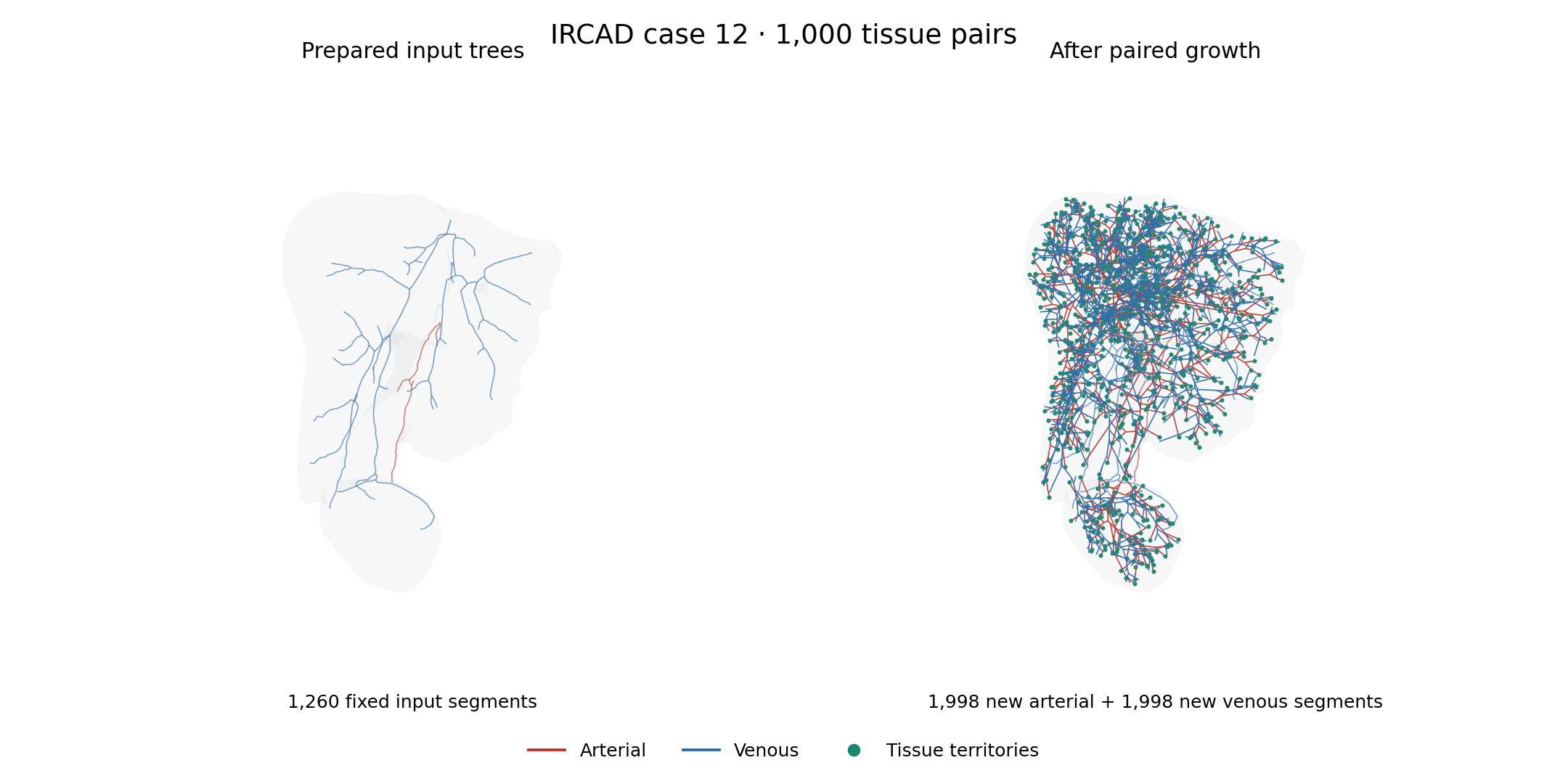
Prepared input trees (left) and the verified 1,000-pair result (right), using the same camera and spatial scale. Red is arterial and blue is venous; green points mark arterial endpoints of the common tissue territories. The gray envelope is the native remeshed tissue. Line widths are for display; physical radii are stored in the output fields. Anatomical source: IRCAD case 12, Soler and coauthors (2010).

Build the application

Use deal.II with its Gmsh API, VTK and simplex support. The standalone growth application does not require the optional 1dsolver library. Run the commands below from the repository root; build-release is the example build directory.

cmake -S . -B build-release -G Ninja \
  -DCMAKE_BUILD_TYPE=Release \
  -DENABLE_COUPLED_PROBLEMS=OFF
cmake --build build-release --target liver_vascular -j 2

Set DEAL_II_DIR if CMake does not find your deal.II installation. Select an MPI compiler wrapper with -DCMAKE_CXX_COMPILER=mpicxx when required by your installation. A Debug build names the executable liver_vascular_debug.

Prepare the IRCAD inputs

The preparation step needs Python, VTK, NumPy and VMTK. The tested environment used Python 3.10, VMTK 1.5.0, VTK 9.2.6 and NumPy 2.2.6. For example, prepare an isolated environment with conda or micromamba:

micromamba create -y -n ircad-prep -c conda-forge \
  python=3.10 vmtk=1.5.0 vtk=9.2.6 numpy=2.2.6
micromamba run -n ircad-prep python scripts/prepare_ircad_liver.py \
  build-release/data/ircad-case12

The output directory must be new. The script downloads only the case’s MESHES_VTK.zip, checks the three source-file SHA-256 hashes, and keeps the original files in raw/. To reuse an existing archive, add --mesh-archive "$MESH_ARCHIVE", where MESH_ARCHIVE names your local copy.

The script writes:

File	Purpose
liver.stl	Closed tissue surface, in metres
arterial.vtk	Rooted arterial 1D mesh with radius and growth-leaf fields
venous.vtk	Rooted venous 1D mesh with the same fields
artery.stl, venacava.stl	Retained vessel surfaces for inspection
provenance.json	Source hashes, units, versions and preparation measurements

The source coordinates are in millimetres. All prepared coordinates and radii are converted to metres. The script selects the largest liver component and cancels two oppositely oriented copies of the same triangle that form a zero-volume fin. It rejects any remaining open or nonmanifold liver edges. The raw source files are unchanged.

VMTK’s approximate network extraction identifies tubular paths and radii. The script keeps the largest connected intrahepatic component of each vessel system, checks that it is a tree, and selects its widest leaf as the root. Disconnected components are listed in provenance.json; they are not added as obstacles in this example. Inspect these choices before adapting the recipe to another anatomy.

Two interior leaves per system are marked for extension. Dense samples near these leaves can put several numerical intervals within one vessel diameter. Treating each interval as a separate physical vessel then blocks a new branch against an older interval of the same tube. The preparation script removes only degree-two samples from the selected tails until the incoming interval is sufficiently long. It preserves the leaf and bifurcation positions and records the maximum geometric deviation. For the tested inputs, this removes eight arterial samples and seven venous samples, with maximum deviations of about 0.817 mm and 1.341 mm respectively.

The resulting input has 176 arterial and 1,084 venous line cells. These are the fixed inputs to the growth calculation, not a claim of exact centerline reconstruction from the medical images.

The IRCAD data use the CC BY-NC-ND 4.0 licence. Keep downloaded meshes, extracted centerlines and physical archives outside the repository. The tutorial includes raster illustrations of the numerical example, with source attribution. Cite Luc Soler and coauthors, 3D image reconstruction for comparison of algorithm database: A patient specific anatomical and medical image database, IRCAD technical report, 2010.

Describe the input trees

Each input is a legacy VTK line mesh with three scalar point-data arrays:

Array	Meaning
Radius	Positive vessel radius in metres
Root	One nonzero leaf: the arterial inlet or venous outlet
Grow	Nonzero on the non-root leaves to extend

The mesh must be connected and acyclic. Line-cell direction need not already follow the flow: the application orients edges from the root toward tissue. Venous geometric orientation is also root-to-tissue; its physical flow is in the opposite direction. Radii interpolate between the two endpoints of each line cell. Viscosity comes from the parameter file.

The application assigns physical node ids from the arterial point indices, then the venous point indices offset by the number of arterial points. These are physical graph identities, not solver block numbers. For the supplied prepared case, the arterial root is node 83 and the venous root is node 177. The reference pressure entries below refer to these roots. If you change the input meshes, update the pressure keys to match their Root fields.

Mesh the tissue and grow both systems

CMake generates the runnable file build-release/data/vascularization/liver.prm from the checked-in template. Its central settings are shown below. Paths in this example are relative to the parameter file:

subsection Liver
  set Arterial grid = ../ircad-case12/arterial.vtk
  set Venous grid = ../ircad-case12/venous.vtk
  set Output directory = ../../test_output/liver-vascularization
  subsection Domain
    set Grid generator = ../ircad-case12/liver.stl
    set Triangulation type = fullydistributed
    subsection Surface mesh
      set Input = auto
      set Target edge length = .012
      set Feature angle = 60
      set Volume cells = tetrahedra
    end
  end
  subsection Vascularization
    subsection Growth
      set Seed length = .003
      set Minimum vessel length = .0002
      set Candidate vessels = 16
      set Local optimization steps = 5
    end
    subsection Sampling
      set Terminal count = 1000
      set Random seed = 23
    end
    subsection Physiology
      set Dynamic viscosity = .004
      set Total new-tissue reference flow = 2e-9
      set Reference pressures = 83:12000,177:2000
      set Minimum radius = .00005
    end
    subsection Venous network
      set Enabled = true
      set Terminal separation = .003
    end
  end
end

Use the generated file for the complete tested controls, including the candidate, optimization and geometry budgets. All lengths here are in metres, pressures in pascals and flow in cubic metres per second.

Domain<3,3> first distinguishes an existing volume from a surface. A surface is read into Triangulation<2,3>; reading it into Triangulation<3,3> does not create a volume. The separate meshing step classifies the surface into Gmsh patches, parametrizes them, creates a closed surface loop and generates the volume. It then transfers the tetrahedra to deal.II before partitioning. See surface domains for the supported input readers and every surface-meshing parameter.

For this surface, a feature angle of 60 degrees allows Gmsh to build valid patch parametrizations; 40 degrees failed in the tested installation. With a 12 mm target edge length the tested mesh had 13,351 tetrahedra and a volume of about 1.515 litres. The cleaned surface encloses about 1.530 litres, so the coarse remeshing changes the enclosed volume by about 0.94%.

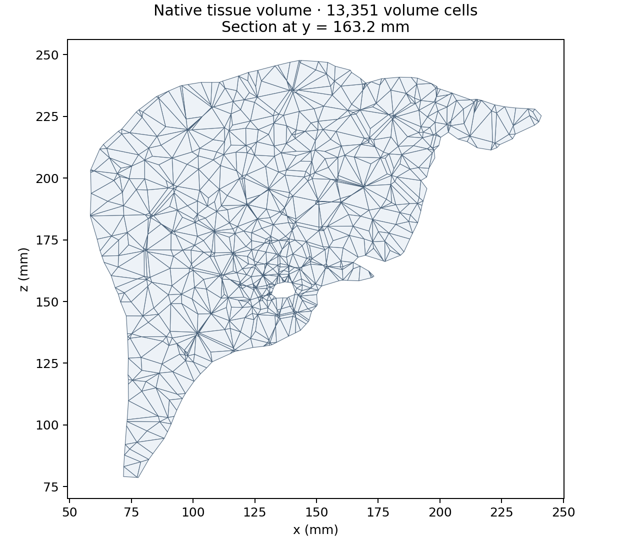
Section at y = 163.2 mm through the exported volume of 13,351 tetrahedra. Polygon edges follow the intersections of the plane with the volume cells. The plot uses the actual native mesh and converts coordinates to millimetres for display.

The arterial generator starts at the marked input leaves and assigns new common tissue territories. The venous generator subsequently extends the marked venous leaves to these territories, with distinct endpoints separated by 3 mm. Each accepted pair receives a positive microvascular resistance. Both growth stages check their new vessel envelopes against the tissue boundary and both vessel systems. Input geometry remains fixed.

The separation must accommodate the endpoint radii. The initial 1 mm trial failed venous startup on this case; 3 mm passed the same geometry checks. Increasing a finite search budget does not make a geometrically blocked connection admissible.

The recipe requests 1,000 common tissue territories, each with one new arterial and one new venous terminal. For a short trial, set Terminal count to 32 and pass --pairs 32 to the checker below.

Run the full recipe in Release on 32 MPI processes, as in the verified 1,000-pair calculation:

mpirun -np 32 build-release/liver_vascular \
  build-release/data/vascularization/liver.prm

For a short two-process trial, set Terminal count = 32 and choose a new output directory in a copy of the parameter file, then run:

mpirun -np 2 build-release/liver_vascular \
  build-release/data/vascularization/liver-mpi.prm

The application resolves relative paths against its parameter file. It can be launched from an unrelated directory. Each run requires a new output directory; an unsuccessful result is not archived as an accepted vascular network.

For hexahedra, change Volume cells to hexahedra. Gmsh still generates the tetrahedral volume first, then Gmsh subdivides each tetrahedron into four conforming hexahedra. The tested liver consequently had 53,404 hexahedra with the same enclosed volume. This is an unstructured hexahedral mesh, not a structured organ-aligned grid. Regenerate and verify the vascular result on the selected background; changing its cells can change sampled growth paths.

Inspect and verify the result

Open liver_0.pvtu and vessels_0.pvtu in ParaView. Give the liver a low opacity and colour the vessel field System: zero is arterial and one is venous. Generated distinguishes fixed imported segments (zero) from new segments (one). Radius is the radius at the numerical interval midpoint, repeated at its patch endpoints. Use it as the point scalar for a varying-radius Tube filter.

The output also contains:

• network/: a native distributed physical archive, including territories and terminal pairs;

• nodes-*.csv and vessels-*.csv: each owned physical record once, with stable integer identifiers, coordinates, radii and provenance;

• terminals-*.csv and pairs-*.csv: common territories, demand and bed resistance;

• summary.csv: global background, vessel and pair counts and vessel volume fraction.

Check the physical result independently of the generator:

micromamba run -n ircad-prep python scripts/check_liver_vascular.py \
  build-release/data/ircad-case12 \
  build-release/test_output/liver-vascularization \
  --pairs 1000 --separation .003 \
  --report build-release/test_output/liver-vascularization/verification.json

The checker compares all supplied nodes, ports, edges and endpoint radii with the exported physical records. It requires growth in both systems, unique arterial–venous pairings, equal paired demand, positive bed resistances and the requested separation. It also samples each new vessel against the exported volume. This sample check supplements the generator’s continuous geometry certification; it does not replace it.

The verified 32-rank Release run produced 1,000 tissue pairs and 5,256 physical vessels: the 1,260 fixed input segments plus 1,998 new arterial and 1,998 new venous segments. The independent check preserved all input nodes, ports, edges and radii and found a positive sampled wall margin for every new vessel. Numerical subdivision of these physical vessels is a separate step and can produce more 1D cells.

The dense recipe uses 16 candidate vessels per insertion; eight candidates exhausted the finite sampling budget on this case. MPI partitions change the sampled growth paths, so another process count can need different search controls. The smaller 32-pair case was also verified on two and four ranks.

Reproduce the illustrations

The published figures come from the checked 32-rank run. Their manifest records the simulation source revision, input and output SHA-256 hashes, software versions, camera, section plane and independent verification results. The anatomical source is 3D-IRCADb-1 case 12, credited to Soler and coauthors (2010) above.

Install Matplotlib in the preparation environment, then render the same views from your own accepted result:

micromamba run -n ircad-prep python -m pip install matplotlib==3.10.9
micromamba run -n ircad-prep python scripts/render_liver_figures.py \
  build-release/data/ircad-case12 \
  build-release/test_output/liver-vascularization \
  build-release/liver-figures --pairs 1000 \
  --source-revision "$(git rev-parse HEAD)"

Pass the revision used to build the simulation binary. The renderer reruns the physical-data checks before plotting and writes two PNGs, a verification report and a manifest. It merges exactly coincident DataOut patch vertices before extracting the tissue exterior. The section preserves quadrilateral cuts of tetrahedra without introducing display diagonals.

A successful growth calculation demonstrates a paired geometric network on this tissue mesh. It does not establish physiological accuracy, resolve capillaries, or guarantee that every point of the liver is adequately served. Use the existing coverage and calibration controls when imposing a service distance or a volume objective.

Add portal inflow

The optional portal network supplies the same territories as the artery; the venous tree drains their combined flow. It is not a partition of the liver into arterial and portal territories.

Prepare a new input directory with the third tree:

micromamba run -n ircad-prep python scripts/prepare_ircad_liver.py \
  build-release/data/ircad-case12-portal --with-portal

This additionally reads MESHES_VTK/portalvein.vtk, a surface in the IRCAD archive, and extracts portal.vtk with the same VMTK procedure. The portal surface is not a usable 1D mesh. The preparation manifest records the source digest, retained component, root and selected leaves. The checked recipe yields 739 portal nodes and two growth leaves. Arterial and venous coordinates, radii and physical identifiers stay the same. With --with-portal, a selected growth endpoint inside another tree’s conservative capsule envelope is disabled in the new input’s Grow array and recorded in the manifest. The recipe disables arterial endpoint 11, which intersects the portal envelope; arterial endpoint 10 remains available. Preparation fails if no selected endpoint remains for any role. The generator still certifies every proposed vessel continuously. Arterial and venous trees are imported before the portal tree so their physical identifiers stay the same. The portal root is then physical node 1262 for this recipe. Recompute these root ids if the preparation settings change.

Copy the generated parameter file for a separate run:

cp build-release/data/vascularization/liver.prm \
  build-release/data/vascularization/liver-portal.prm

Use the new prepared directory for all three line meshes and the liver surface. Edit the copied file’s existing subsections with these settings. The application default remains 1,000 territories per network; this shorter trial requests 32:

subsection Liver
  set Arterial grid = ../ircad-case12-portal/arterial.vtk
  set Venous grid = ../ircad-case12-portal/venous.vtk
  set Portal grid = ../ircad-case12-portal/portal.vtk
  set Output directory = ../../test_output/liver-portal
  subsection Domain
    set Grid generator = ../ircad-case12-portal/liver.stl
  end
  subsection Vascularization
    subsection Sampling
      set Terminal count = 32
    end
    subsection Physiology
      set Reference pressures = 83:12000,177:2000,1262:5000
    end
    subsection Portal network
      set Enabled = true
      set Terminal separation = .004
      set Flow fraction = .7
    end
  end
end

Save the parameter file in build-release/data/vascularization, as in the two-network example. All paths are relative to that file. Keep the venous network enabled. The total new-tissue flow now denotes venous drainage: with the illustrative fraction 0.7, portal inflow supplies 70% and arterial inflow 30%. These values and root pressures are modeling inputs. Leave Compartment resistances at its three zero defaults to derive positive arms using a common pressure between the venous terminal pressure and both supplying terminal pressures. The final solve checks each requested supply and drainage, including Q_v = Q_a + Q_p. See three-network reference flow for the equations and supplied-resistance alternative.

The CSV output includes triplets-*.csv with terminal identities, three arm resistances, actual supply and drainage flows and the common pressure. In VTK, System values remain 0=arterial, 1=venous, with 2=portal. The physical archive retains all three roles and their common compartments. Existing arterial–venous parameter files retain their original behavior.

Run the copied parameter file:

mpirun -np 4 build-release/liver_vascular \
  build-release/data/vascularization/liver-portal.prm

The verified four-rank Release run with deal.II 9.7.1 produced 32 triplets, 2,185 physical vessels and 11,047 tissue cells. It retained 2,001 input nodes and 1,998 input segments, and added 63 arterial, 62 portal and 62 venous segments. The independent checker preserved all input coordinates, ports and radii, verified the requested supply split and found a positive sampled wall margin for every new vessel.

This 32-territory trial provides a shorter starting point. A different count or MPI partition can need different search settings; fewer territories do not guarantee an admissible initial connection for every selected attachment. The published 1,000-pair run and its figures above remain the arterial–venous reference. To check a three-network run, pass --triplets N instead of --pairs N, together with the portal separation:

micromamba run -n ircad-prep python scripts/check_liver_vascular.py \
  build-release/data/ircad-case12-portal build-release/test_output/liver-portal \
  --triplets 32 --separation .003 --portal-separation .004 \
  --portal-flow-fraction .7

The figure renderer accepts the same three options and colors portal vessels purple. Geometry certification, demand matching and positive perfusion are required before writing an accepted result; the finite growth budget can fail for an incompatible geometry or search configuration.

Save the volume and reuse the physical network

To save the exact generated volume before distributed partitioning, set:

subsection Liver
  set Write volume mesh = true
end

The new output directory then contains liver.msh as well as the physical network/ archive. Set Only generate mesh = true to stop after writing the volume, for example when preparing several tissue resolutions. This mode also requires Write volume mesh = true. It does not generate or validate a vascular network. The ordinary growth path remains the default.

With a compatible MetricFlowX package, metric_flow_x_elastodynamics can load the physical archive and subdivide its vessels against its final tissue mesh. The imported tissue mesh can be liver.msh; select a fully distributed Domain for tetrahedra. Configure the ordinary solid, IDA, inflow and lift parameters, then add the following explicit vascular data:

subsection MetricFlowX coupling
  subsection Archived network
    set Directory = /absolute/path/to/network
    set Young moduli = 400000,400000,400000
    set Wall thickness ratios = .1,.1,.1
    set Reference pressures = 10064.5,629.6,1066.6
    set Portal pressure = 1066.6
    set Venous pressure = 629.6
    set Root resistance = 100000
  end
end

The three material entries are in arterial, venous, portal order. Young moduli and reference pressures are in Pa; wall thickness is the given ratio times the mean vessel radius. Root resistance is in Pa s/m³. The numbers above illustrate the parameter contract, not a patient calibration. The arterial root retains the native inflow function or CSV. Portal and venous roots use separate pressure reservoirs with the stated positive series resistance. This requires a backend with orientation-correct RCR conditions at both vessel ends. The saved common microvascular compartments connect the tissue leaves; they do not acquire extra independent outlet resistances. An archive with unconnected tissue leaves is rejected by default. In particular, the anatomical growth example above retains unused input leaves. To declare selected ends closed, set Sealed input terminal ids under the same Archived network subsection to their comma-separated physical Terminal IDs. Every remaining tissue leaf must belong to a saved bed, and a bed terminal cannot also be sealed. This needs the native sealed-endpoint API from MetricFlowX #88 and a matching rebuild. A sealed end has exactly zero flow and adds no reservoir; it is an explicit model assumption and must not count as a perfused terminal.

The coupled output reports each block’s DoFs and the total. Per-rank mesh_scale-*.csv files retain each numerical interval’s length and the minimum/maximum diameter of crossed tissue cells. Short-cell exceptions are reported explicitly. Terminal CSV diagnostics use actual boundary traces, including the coupled external pressure. Mass diagnostics compare net outward flow with volume change between accepted output times; the first record has no previous interval.

For an equilibrium start, IDA’s Correction type at initial time = use_y_dot uses a zero state derivative to solve the complete coupled residual at the initial time. This equilibrates the chosen boundary data; it does not establish a periodic coupled state. For exterior tissue support, configure the solid’s Robin boundary ids, Functions/Robin coefficient and Functions/Robin boundary as described in the Robin boundary reference.

Coupled error control can use different absolute tolerances for quantities with different units. Set Displacement absolute tolerance (m), Velocity absolute tolerance (m/s), and Wall pressure absolute tolerance (Pa) under MetricFlowX coupling. Their zero defaults retain the common IDA absolute tolerance. Use native flow tolerances = true reuses MetricFlowX’s Area absolute tolerance fraction, Velocity absolute tolerance, and Capacitor pressure absolute tolerance for its mixed area/velocity/pressure vector. This delegates component numbering and reference-area scaling to MetricFlowX. Choose and verify these tolerances against the spatial and temporal errors of the intended case.

The coupled IRCAD12 starting case provides a two-territory arterial/portal/venous archive and four run profiles. Its research release contains the generated meshes, parameters, numerical inputs/results and a literature report. The million and ten-million profiles are preparation cases; their transient solver performance is not validated.

For an archived liver case, Stop at output times = true under /MetricFlowX coupling/ ends an internal IDA step at each saved time. The default remains dense output. Internal stops retain the BDF history and avoid interpolation defects in nonlinear hydraulic constraints. Control Newton convergence separately through the IDA Nonlinear solver subsection.