Elasticity¶

This tutorial explains the ElasticityProblem application in the simplest setting: bulk elasticity without immersed inclusions.

The examples present exact-solution convergence tests, using the method of manufactured solutions (MMS) for both static and dynamic cases. The five test files are:

tutorials/elasticity/strong_dirichlet.prm
tutorials/elasticity/weak_dirichlet.prm
tutorials/elasticity/neumann.prm
tutorials/elasticity/dynamic_purely_elastic.prm
tutorials/elasticity/damped_kv_dispersion.prm

All these tests run with empty Immersed inclusions sections, so they isolate the behavior of the background elasticity solver, boundary conditions, and time integration.

What Problem Is Solved?¶

The code solves linear elasticity in a domain \(\Omega\) (here, the unit square), for the displacement field

\[u : \Omega \times [0,T] \to \mathbb{R}^{d}.\]

In the no-inclusion configuration used in this tutorial, the model is the classical bulk problem:

\[\rho\,\partial_{tt}u - \nabla\cdot\sigma(u,\partial_t u) = f \qquad \text{in } \Omega,\]

with boundary conditions chosen test by test (strong Dirichlet, weak Dirichlet/Nitsche-like penalty, and mixed Dirichlet-Neumann), and with material parameters from Material properties.

For the static tests, Final time = 0.0, so the run reduces to a stationary solve with manufactured source and exact solution. For the dynamic tests, time-stepping is active and the exact solution is used to verify both space and time behavior.

Where The Implementation Lives¶

Main files:

apps/app_elasticity.cc
include/elasticity.h
source/elasticity.cc
include/elasticity_problem_parameters.h
source/elasticity_problem_parameters.cc

How to run:

./build/elasticity[_debug] ../tutorials/elasticity/<input_file.prm>

Dimension selection follows app_elasticity.cc filename conventions:

filenames containing 23d instantiate ElasticityProblem<2,3>;
filenames containing 3d instantiate ElasticityProblem<3>;
otherwise it instantiates ElasticityProblem<2>.

The five tutorial files in this page are 2D cases.

Common Structure Of The Test Files¶

Across the five files, you will repeatedly find:

subsection Error: enables error tables and convergence-rate reporting;
subsection Functions: manufactured exact solution, boundary data, right-hand side, and initial conditions;
subsection Immersed Problem: FE degree, mesh generation, refinement cycles, material parameters, BC IDs, and time settings;
empty Immersed inclusions data, meaning no reduced coupling is active.

In all convergence runs, the error file records norms (typically L2_norm, H1_norm, and Linfty_norm) as functions of mesh size or DoFs.

Test 1: Strong Dirichlet (Static MMS)¶

File: tutorials/elasticity/strong_dirichlet.prm

Goal:

verify spatial convergence for a static manufactured solution;
impose displacement strongly on all boundaries (Dirichlet boundary ids = 0,1,2,3).

Exact solution (component-wise) is explicitly prescribed in Functions/Exact solution:

\[\begin{split}\begin{aligned} u_1(x,y,t) &= x y (x-1)(y-1) + \sin(\pi x)\sin(\pi y)\cos\!\left(\tfrac{5\pi t}{2}\right), \\ u_2(x,y,t) &= x y (x-1)(y-1) + \sin\!\left(\tfrac{5\pi t}{2}\right)\sin(\pi y)\cos(\pi x). \end{aligned}\end{split}\]

At Final time = 0.0, this is effectively a static consistency check of the assembled bulk operator against the manufactured forcing.

Constitutive law and constants:

\[\sigma(u) = 2\mu\,\varepsilon(u) + \lambda\,\operatorname{tr}(\varepsilon(u)) I, \qquad \varepsilon(u)=\tfrac12(\nabla u + \nabla u^T).\]

For this test, the constants are:

\(\lambda = 2.0\), from Immersed Problem/Material properties/default/Lame lambda;
\(\mu = 1.0\), from Immersed Problem/Material properties/default/Lame mu;
\(\eta = 0.0\), from Immersed Problem/Material properties/default/Viscosity eta, so no viscous contribution is active;
\(\rho = 0.0\), from Immersed Problem/Material properties/default/Density, which is consistent with the static solve;
there are no additional Function constants in this test: the manufactured coefficients appear directly in Functions/Exact solution, Functions/Initial displacement, Functions/Initial velocity, and Functions/Right hand side.

subsection Error
  set Enable computation of the errors = true
  set Error file name                  = static_convergence/errors_strong_dirichlet.txt
  set Error precision                  = 8
  set Exponent for p-norms             = 2
  set Extra columns                    = cells, dofs
  set List of error norms to compute   = L2_norm, Linfty_norm, H1_norm
  set Rate key                         = dofs
  set Rate mode                        = reduction_rate_log2
end
subsection Functions
  subsection Dirichlet boundary conditions
    set Function constants  =
    set Function expression = x*y*(x - 1)*(y - 1) + sin(pi*x)*sin(pi*y)*cos(5*pi*t/2); x*y*(x - 1)*(y - 1) + sin(5*pi*t/2)*sin(pi*y)*cos(pi*x)
    set Variable names      = x,y,t
  end
  subsection Exact solution
    set Function constants  =
    set Function expression = x*y*(x - 1)*(y - 1) + sin(pi*x)*sin(pi*y)*cos(5*pi*t/2); x*y*(x - 1)*(y - 1) + sin(5*pi*t/2)*sin(pi*y)*cos(pi*x)
    set Variable names      = x,y,t
  end
  subsection Initial displacement
    set Function constants  =
    set Function expression = x*y*(x - 1)*(y - 1) + sin(pi*x)*sin(pi*y)*cos(5*pi*t/2); x*y*(x - 1)*(y - 1) + sin(5*pi*t/2)*sin(pi*y)*cos(pi*x)
    set Variable names      = x,y,t
  end
  subsection Initial velocity
    set Function constants  =
    set Function expression = -5*pi*sin(5*pi*t/2)*sin(pi*x)*sin(pi*y)/2; 5*pi*sin(pi*y)*cos(5*pi*t/2)*cos(pi*x)/2
    set Variable names      = x,y,t
  end
  subsection Neumann boundary conditions
    set Function constants  =
    set Function expression = 0; 0
    set Variable names      = x,y,t
  end
  subsection Right hand side
    set Function constants  =
    set Function expression = -2.0*x^2 - 12.0*x*y + 8.0*x - 8.0*y^2 + 14.0*y + 3.0*pi^2*sin(5*pi*t/2)*sin(pi*x)*cos(pi*y) + 5.0*pi^2*sin(pi*x)*sin(pi*y)*cos(5*pi*t/2) - 3.0; -8.0*x^2 - 12.0*x*y + 14.0*x - 2.0*y^2 + 8.0*y + 5.0*pi^2*sin(5*pi*t/2)*sin(pi*y)*cos(pi*x) - 3.0*pi^2*cos(5*pi*t/2)*cos(pi*x)*cos(pi*y) - 3.0
    set Variable names      = x,y,t
  end
end
subsection Immersed Problem
  set Dirichlet boundary ids             = 0,1,2,3
  set Weak Dirichlet boundary ids      = 
  set FE degree                          = 1
  set Initial refinement                 = 2
  set Neumann boundary ids               =
  set Normal flux boundary ids           =
  set Output directory                   = static_convergence
  set Output name                        = strong_dirichlet
  set Output pressure                    = false
  set Output results also before solving = false
  set Pressure coupling                  = false
  set Weak Dirichlet penalty coefficient = 100
  subsection Grid generation
    set Domain type              = generate
    set Grid generator           = hyper_cube
    set Grid generator arguments = 0: 1: true
  end
  subsection Immersed inclusions
    set Bounding boxes extraction level   = 1
    set Data file                         =
    set Inclusions                        =
    set Inclusions file                   =
    set Inclusions refinement             = 100
    set Number of fourier coefficients    = 1
    set Reference inclusion data          =
    set Selection of Fourier coefficients =
    subsection Boundary data
      set Function constants   =
      set Function expression  = 0; 0
      set Modulation frequency = 0
      set Variable names       = x,y,t
    end
  end
  subsection Material properties
    set Material tags by material id =
    subsection default
      set Density         = 0.0
      set Lame lambda     = 2.0
      set Lame mu         = 1.0
      set Rayleigh alpha  = 0
      set Rayleigh beta   = 0
      set Viscosity eta   = 0.0
    end
  end
  subsection Refinement and remeshing
    set Coarsening fraction         = 0
    set Maximum number of cells     = 20000
    set Number of refinement cycles = 6
    set Refinement fraction         = 0.3
    set Strategy                    = global
  end
  subsection Time dependency
    set Final time    = 0.0
    set Initial time  = 0.0
    set Newmark beta  = 0.25
    set Newmark gamma = 0.5
    set Time step     = 0.005
  end
end
subsection Solvers
  subsection Augmented Lagrange
    set Log frequency = 1
    set Log history   = false
    set Log result    = true
    set Max steps     = 100
    set Reduction     = 1.e-10
    set Tolerance     = 1.e-10
  end
  subsection Displacement
    set Log frequency = 1
    set Log history   = false
    set Log result    = true
    set Max steps     = 100
    set Reduction     = 1.e-10
    set Tolerance     = 1.e-10
  end
  subsection Reduced mass
    set Log frequency = 1
    set Log history   = false
    set Log result    = true
    set Max steps     = 100
    set Reduction     = 1.e-10
    set Tolerance     = 1.e-10
  end
  subsection Schur complement
    set Log frequency = 1
    set Log history   = false
    set Log result    = true
    set Max steps     = 100
    set Reduction     = 1.e-10
    set Tolerance     = 1.e-10
  end
end

Test 2: Weak Dirichlet (Static MMS)¶

File: tutorials/elasticity/weak_dirichlet.prm

Goal:

test the weak imposition of Dirichlet data through penalty terms;
compare with the same exact field of Test 1.

Key differences from strong Dirichlet:

Dirichlet boundary ids is empty;
Weak Dirichlet boundary ids = 0,1,2,3;
Weak Dirichlet penalty coefficient = 100.

So this test isolates the weak boundary treatment while keeping the same exact solution and forcing.

Constitutive law and constants:

\[\sigma(u) = 2\mu\,\varepsilon(u) + \lambda\,\operatorname{tr}(\varepsilon(u)) I, \qquad \varepsilon(u)=\tfrac12(\nabla u + \nabla u^T).\]

The constants are the same as in Test 1 and are read from the same block:

\(\lambda = 2.0\), from Immersed Problem/Material properties/default/Lame lambda;
\(\mu = 1.0\), from Immersed Problem/Material properties/default/Lame mu;
\(\eta = 0.0\), from Immersed Problem/Material properties/default/Viscosity eta;
\(\rho = 0.0\), from Immersed Problem/Material properties/default/Density;
no symbolic Function constants are used; all coefficients are written directly in the Functions/*/Function expression entries.

subsection Error
  set Enable computation of the errors = true
  set Error file name                  = static_convergence/errors_weak_dirichlet.txt
  set Error precision                  = 8
  set Exponent for p-norms             = 2
  set Extra columns                    = cells, dofs
  set List of error norms to compute   = L2_norm, Linfty_norm, H1_norm
  set Rate key                         = dofs
  set Rate mode                        = reduction_rate_log2
end
subsection Functions
  subsection Dirichlet boundary conditions
    set Function constants  =
    set Function expression = x*y*(x - 1)*(y - 1) + sin(pi*x)*sin(pi*y)*cos(5*pi*t/2); x*y*(x - 1)*(y - 1) + sin(5*pi*t/2)*sin(pi*y)*cos(pi*x)
    set Variable names      = x,y,t
  end
  subsection Exact solution
    set Function constants  =
    set Function expression = x*y*(x - 1)*(y - 1) + sin(pi*x)*sin(pi*y)*cos(5*pi*t/2); x*y*(x - 1)*(y - 1) + sin(5*pi*t/2)*sin(pi*y)*cos(pi*x)
    set Variable names      = x,y,t
  end
  subsection Initial displacement
    set Function constants  =
    set Function expression = x*y*(x - 1)*(y - 1) + sin(pi*x)*sin(pi*y)*cos(5*pi*t/2); x*y*(x - 1)*(y - 1) + sin(5*pi*t/2)*sin(pi*y)*cos(pi*x)
    set Variable names      = x,y,t
  end
  subsection Initial velocity
    set Function constants  =
    set Function expression = -5*pi*sin(5*pi*t/2)*sin(pi*x)*sin(pi*y)/2; 5*pi*sin(pi*y)*cos(5*pi*t/2)*cos(pi*x)/2
    set Variable names      = x,y,t
  end
  subsection Neumann boundary conditions
    set Function constants  =
    set Function expression = 0; 0
    set Variable names      = x,y,t
  end
  subsection Right hand side
    set Function constants  =
    set Function expression = -2.0*x^2 - 12.0*x*y + 8.0*x - 8.0*y^2 + 14.0*y + 3.0*pi^2*sin(5*pi*t/2)*sin(pi*x)*cos(pi*y) + 5.0*pi^2*sin(pi*x)*sin(pi*y)*cos(5*pi*t/2) - 3.0; -8.0*x^2 - 12.0*x*y + 14.0*x - 2.0*y^2 + 8.0*y + 5.0*pi^2*sin(5*pi*t/2)*sin(pi*y)*cos(pi*x) - 3.0*pi^2*cos(5*pi*t/2)*cos(pi*x)*cos(pi*y) - 3.0
    set Variable names      = x,y,t
  end
end
subsection Immersed Problem
  set Dirichlet boundary ids             = 
  set Weak Dirichlet boundary ids        = 0,1,2,3
  set FE degree                          = 1
  set Initial refinement                 = 2
  set Neumann boundary ids               =
  set Normal flux boundary ids           =
  set Output directory                   = static_convergence
  set Output name                        = weak_dirichlet
  set Output pressure                    = false
  set Output results also before solving = false
  set Pressure coupling                  = false
  set Weak Dirichlet penalty coefficient = 100
  subsection Grid generation
    set Domain type              = generate
    set Grid generator           = hyper_cube
    set Grid generator arguments = 0: 1: true
  end
  subsection Immersed inclusions
    set Bounding boxes extraction level   = 1
    set Data file                         =
    set Inclusions                        =
    set Inclusions file                   =
    set Inclusions refinement             = 100
    set Number of fourier coefficients    = 1
    set Reference inclusion data          =
    set Selection of Fourier coefficients =
    subsection Boundary data
      set Function constants   =
      set Function expression  = 0; 0
      set Modulation frequency = 0
      set Variable names       = x,y,t
    end
  end
  subsection Material properties
    set Material tags by material id =
    subsection default
      set Density         = 0.0
      set Lame lambda     = 2.0
      set Lame mu         = 1.0
      set Rayleigh alpha  = 0
      set Rayleigh beta   = 0
      set Viscosity eta   = 0.0
    end
  end
  subsection Refinement and remeshing
    set Coarsening fraction         = 0
    set Maximum number of cells     = 20000
    set Number of refinement cycles = 6
    set Refinement fraction         = 0.3
    set Strategy                    = global
  end
  subsection Time dependency
    set Final time    = 0.0
    set Initial time  = 0.0
    set Newmark beta  = 0.25
    set Newmark gamma = 0.5
    set Time step     = 0.005
  end
end
subsection Solvers
  subsection Augmented Lagrange
    set Log frequency = 1
    set Log history   = false
    set Log result    = true
    set Max steps     = 100
    set Reduction     = 1.e-10
    set Tolerance     = 1.e-10
  end
  subsection Displacement
    set Log frequency = 1
    set Log history   = false
    set Log result    = true
    set Max steps     = 100
    set Reduction     = 1.e-10
    set Tolerance     = 1.e-10
  end
  subsection Reduced mass
    set Log frequency = 1
    set Log history   = false
    set Log result    = true
    set Max steps     = 100
    set Reduction     = 1.e-10
    set Tolerance     = 1.e-10
  end
  subsection Schur complement
    set Log frequency = 1
    set Log history   = false
    set Log result    = true
    set Max steps     = 100
    set Reduction     = 1.e-10
    set Tolerance     = 1.e-10
  end
end

Test 3: Mixed Dirichlet-Neumann (Static MMS)¶

File: tutorials/elasticity/neumann.prm

Goal:

verify the handling of mixed boundary conditions;
keep an exact manufactured solution and consistent traction on a Neumann side.

Boundary setup:

Dirichlet boundary ids = 0,2,3;
Neumann boundary ids = 1.

The Neumann data in Neumann boundary conditions is chosen to match the exact solution and constitutive law, so the whole setup remains analytically consistent.

Constitutive law and constants:

\[\sigma(u) = 2\mu\,\varepsilon(u) + \lambda\,\operatorname{tr}(\varepsilon(u)) I, \qquad \varepsilon(u)=\tfrac12(\nabla u + \nabla u^T).\]

The constants are:

\(\lambda = 2\), from Immersed Problem/Material properties/default/Lame lambda;
\(\mu = 1\), from Immersed Problem/Material properties/default/Lame mu;
\(\eta = 0\), from Immersed Problem/Material properties/default/Viscosity eta;
\(\rho = 0\), from Immersed Problem/Material properties/default/Density;
no Function constants are declared; the manufactured displacement, body force, and Neumann traction are written explicitly in Functions/Exact solution, Functions/Right hand side, and Functions/Neumann boundary conditions.

In particular, the traction on boundary id 1 is the one induced by this \(\sigma(u)\) and the manufactured exact solution, and it is stored in Functions/Neumann boundary conditions/Function expression.

subsection Error
  set Enable computation of the errors = true
  set Error file name                  = static_convergence/errors_neumann.txt
  set Error precision                  = 8
  set Exponent for p-norms             = 2
  set Extra columns                    = cells, dofs
  set List of error norms to compute   = L2_norm, Linfty_norm, H1_norm
  set Rate key                         = dofs
  set Rate mode                        = reduction_rate_log2
end
subsection Functions
  subsection Dirichlet boundary conditions
    set Function constants   =
    set Function expression  = x*y*(x - 1)*(y - 1) + sin(pi*x)*sin(pi*y); x*y*(x - 1)*(y - 1) + sin(pi*y)*cos(pi*x)
    set Modulation frequency = 0
    set Variable names       = x,y,t
  end
  subsection Exact solution
    set Function constants  =
    set Function expression = x*y*(x - 1)*(y - 1) + sin(pi*x)*sin(pi*y); x*y*(x - 1)*(y - 1) + sin(pi*y)*cos(pi*x)
    set Variable names      = x,y,t
    set Weight expression   = 1.
  end
  subsection Initial displacement
    set Function constants  =
    set Function expression = x*y*(x - 1)*(y - 1) + sin(pi*x)*sin(pi*y); x*y*(x - 1)*(y - 1) + sin(pi*y)*cos(pi*x)
    set Variable names      = x,y,t
  end
  subsection Initial velocity
    set Function constants  =
    set Function expression = 0; 0
    set Variable names      = x,y,t
  end
  subsection Neumann boundary conditions
    set Function constants   =
    set Function expression  = 4*x^2*y - 2*x^2 + 8*x*y^2 - 12*x*y + 2*x - 4*y^2 + 4*y + 4*pi*sin(pi*y)*cos(pi*x) + 2*pi*cos(pi*x)*cos(pi*y); 2*x^2*y - x^2 + 2*x*y^2 - 4*x*y + x - y^2 + y + sqrt(2)*pi*sin(pi*x)*cos(pi*(y + 1/4))
    set Modulation frequency = 0
    set Variable names       = x,y,t
  end
  subsection Right hand side
    set Function constants   =
    set Function expression  = -2*x^2 - 12*x*y + 8*x - 8*y^2 + 14*y + 5*pi^2*sin(pi*x)*sin(pi*y) + 3*pi^2*sin(pi*x)*cos(pi*y) - 3; -8*x^2 - 12*x*y + 14*x - 2*y^2 + 8*y + 5*pi^2*sin(pi*y)*cos(pi*x) - 3*pi^2*cos(pi*x)*cos(pi*y) - 3
    set Modulation frequency = 0
    set Variable names       = x,y,t
  end
end
subsection Immersed Problem
  set Dirichlet boundary ids             = 0,2,3
  set FE degree                          = 1
  set Initial refinement                 = 1
  set Neumann boundary ids               = 1
  set Normal flux boundary ids           =
  set Output directory                   = static_convergence
  set Output name                        = neumann
  set Output pressure                    = false
  set Output results also before solving = false
  set Pressure coupling                  = false
  set Weak Dirichlet boundary ids        = 
  set Weak Dirichlet penalty coefficient = 1000
  subsection Grid generation
    set Domain type              = generate
    set Grid generator           = hyper_cube
    set Grid generator arguments = 0: 1: true
  end
  subsection Immersed inclusions
    set Bounding boxes extraction level   = 1
    set Data file                         =
    set Inclusions                        =
    set Inclusions file                   =
    set Inclusions refinement             = 100
    set Number of fourier coefficients    = 1
    set Reference inclusion data          =
    set Selection of Fourier coefficients =
    subsection Boundary data
      set Function constants   =
      set Function expression  = 0; 0
      set Modulation frequency = 0
      set Variable names       = x,y,t
    end
  end
  subsection Material properties
    set Material tags by material id =
    subsection default
      set Density         = 0
      set Lame lambda     = 2
      set Lame mu         = 1
      set Rayleigh alpha  = 0
      set Rayleigh beta   = 0
      set Viscosity eta   = 0
    end
  end
  subsection Refinement and remeshing
    set Coarsening fraction         = 0
    set Maximum number of cells     = 20000
    set Number of refinement cycles = 6
    set Refinement fraction         = 0.3
    set Strategy                    = global
  end
  subsection Time dependency
    set Final time    = 0
    set Initial time  = 0
    set Newmark beta  = 0.25
    set Newmark gamma = 0.5
    set Time step     = 0.005
  end
end
subsection Solvers
  subsection Augmented Lagrange
    set Log frequency = 1
    set Log history   = false
    set Log result    = true
    set Max steps     = 100
    set Reduction     = 1.e-10
    set Tolerance     = 1.e-10
  end
  subsection Displacement
    set Log frequency = 1
    set Log history   = false
    set Log result    = true
    set Max steps     = 100
    set Reduction     = 1.e-10
    set Tolerance     = 1.e-10
  end
  subsection Reduced mass
    set Log frequency = 1
    set Log history   = false
    set Log result    = true
    set Max steps     = 100
    set Reduction     = 1.e-10
    set Tolerance     = 1.e-10
  end
  subsection Schur complement
    set Log frequency = 1
    set Log history   = false
    set Log result    = true
    set Max steps     = 100
    set Reduction     = 1.e-10
    set Tolerance     = 1.e-10
  end
end

Test 4: Dynamic Purely Elastic Wave (No Viscosity)¶

File: tutorials/elasticity/dynamic_purely_elastic.prm

Goal:

test transient behavior with \(\eta = 0\) (pure elasticity);
verify wave propagation against a known analytic traveling-wave solution.

Material block sets:

Density = 1.0
Lame lambda = 2.0
Lame mu = 1.0
Viscosity eta = 0.0

The exact displacement is a 1D-in-space sinusoidal wave in the first component, with matching initial velocity and forcing.

Constitutive law and constants:

\[\sigma(u) = 2\mu\,\varepsilon(u) + \lambda\,\operatorname{tr}(\varepsilon(u)) I, \qquad \varepsilon(u)=\tfrac12(\nabla u + \nabla u^T).\]

The material constants used by the solver are:

\(\rho = 1.0\), from Immersed Problem/Material properties/default/Density;
\(\lambda = 2.0\), from Immersed Problem/Material properties/default/Lame lambda;
\(\mu = 1.0\), from Immersed Problem/Material properties/default/Lame mu;
\(\eta = 0.0\), from Immersed Problem/Material properties/default/Viscosity eta.

The same values are also repeated symbolically in the Functions/*/Function constants entries as:

lam = 2.0
mu0 = 1.0
eta0 = 0.0
rho0 = 1.0

These function-side constants are used inside the analytic formulas in Functions/Exact solution, Functions/Initial displacement, Functions/Initial velocity, and Functions/Right hand side.

subsection Error
  set Error file name = dynamic_convergence/errors_purely_elastic.txt
  set Error precision = 8
end
subsection Functions
  subsection Dirichlet boundary conditions
    set Function constants  = lam=2.0, mu0=1.0, eta0=0.0, rho0=1.0
    set Function expression = -0.2*sin(pi*(6.06060606060606*t*sqrt((lam + 2*mu0)/rho0) - 6.06060606060606*x)); 0
  end
  subsection Exact solution
    set Function constants  = lam=2.0, mu0=1.0, eta0=0.0, rho0=1.0
    set Function expression = -0.2*sin(pi*(6.06060606060606*t*sqrt((lam + 2*mu0)/rho0) - 6.06060606060606*x)); 0
  end
  subsection Initial displacement
    set Function constants  = lam=2.0, mu0=1.0, eta0=0.0, rho0=1.0
    set Function expression = -0.2*sin(pi*(6.06060606060606*t*sqrt((lam + 2*mu0)/rho0) - 6.06060606060606*x)); 0
  end
  subsection Initial velocity
    set Function constants  = lam=2.0, mu0=1.0, eta0=0.0, rho0=1.0
    set Function expression = -1.21212121212121*pi*sqrt((lam + 2*mu0)/rho0)*cos(pi*(6.06060606060606*t*sqrt((lam + 2*mu0)/rho0) - 6.06060606060606*x)); 0
  end
  subsection Neumann boundary conditions
    set Function expression = 0; 0
  end
  subsection Right hand side
    set Function constants  = lam=2.0, mu0=1.0, eta0=0.0, rho0=1.0
    set Function expression = pi^2*(7.34618916437098*lam + 14.692378328742*mu0 - 29.3847566574839*rho0)*sin(pi*(6.06060606060606*t*sqrt((lam + 2*mu0)/rho0) - 6.06060606060606*x))/rho0; 0
  end
end
subsection Immersed Problem
  set Dirichlet boundary ids             =
  set Initial refinement                 = 4
  set Output directory                   = dynamic_convergence
  set Output name                        = purely_elastic
  set Weak Dirichlet boundary ids        = 0,1,2,3
  set Weak Dirichlet penalty coefficient = 1000
  subsection Grid generation
    set Grid generator arguments = 0: 1: true
  end
  subsection Immersed inclusions
    subsection Boundary data
      set Function expression = 0; 0
    end
  end
  subsection Material properties
    subsection default
      set Density       = 1.0
      set Lame lambda   = 2.0
      set Lame mu       = 1.0
      set Viscosity eta = 0.0
    end
  end
  subsection Refinement and remeshing
    set Number of refinement cycles = 4
    set Strategy                    = global
  end
  subsection Time dependency
    set Final time       = .25
    set Initial time     = 0.0
    set Refine time step = true
    set Time step        = 0.0125
  end
end
subsection Solvers
  subsection Augmented Lagrange
    set Reduction = 1.e-10
  end
  subsection Displacement
    set Reduction = 1.e-10
  end
  subsection Reduced mass
    set Reduction = 1.e-10
  end
  subsection Schur complement
    set Reduction = 1.e-10
  end
end

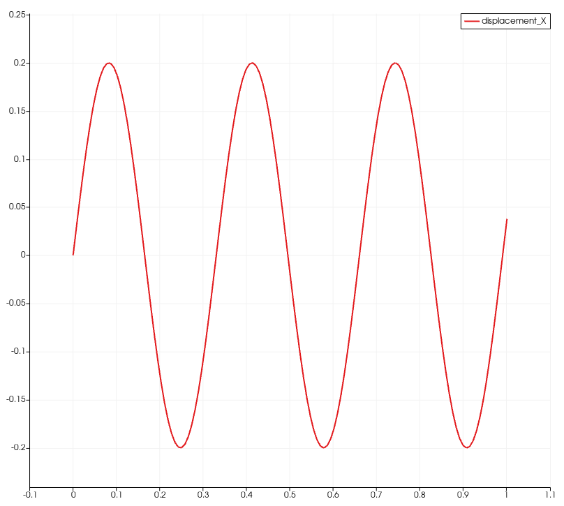
../_images/dynamic_purely_elastic.gif — Displacement field evolution for the undamped traveling-wave manufactured solution.¶

Test 5: Damped Kelvin-Voigt Dispersion¶

File: tutorials/elasticity/damped_kv_dispersion.prm

Goal:

validate dissipative dynamics with Kelvin-Voigt viscosity;
reproduce a damped dispersive harmonic wave profile.

Material block sets Viscosity eta = 0.1, and the exact solution has the form:

\[u_1(x,t) = A\,e^{-k_i x}\sin(k_r x - \omega t), \qquad u_2(x,t)=0,\]

with constants defined in Function constants. This test is useful to check attenuation and phase behavior in time-dependent runs.

Constitutive law and constants:

\[\sigma(u,\dot u) = 2\mu\,\varepsilon(u) + \lambda\,\operatorname{tr}(\varepsilon(u)) I + \eta\,\varepsilon(\dot u), \qquad \varepsilon(v)=\tfrac12(\nabla v + \nabla v^T).\]

The solver-side material constants are:

\(\rho = 1.0\), from Immersed Problem/Material properties/default/Density;
\(\lambda = 2.0\), from Immersed Problem/Material properties/default/Lame lambda;
\(\mu = 1.0\), from Immersed Problem/Material properties/default/Lame mu;
\(\eta = 0.1\), from Immersed Problem/Material properties/default/Viscosity eta.

The analytic wave parameters are listed in the Functions/*/Function constants entries:

lam = 2.0, mu0 = 1.0, eta0 = 0.1, rho0 = 1.0;
a = 0.2;
omega = 12.566370614359172;
kr = 6.066118580856262;
ki = 0.9304459659323195.

These appear in Functions/Dirichlet boundary conditions, Functions/Exact solution, Functions/Initial displacement, Functions/Initial velocity, and Functions/Right hand side.

subsection Error
  set Error file name = dynamic_convergence/errors_damped_kv.txt
  set Error precision = 8
end
subsection Functions
  subsection Dirichlet boundary conditions
    set Function constants  = lam=2.0, mu0=1.0, eta0=0.1, rho0=1.0, a=0.2, omega=12.566370614359172, kr=6.066118580856262, ki=0.9304459659323195
    set Function expression = a*exp(-ki*x)*sin(kr*x - omega*t); 0
  end
  subsection Exact solution
    set Function constants  = lam=2.0, mu0=1.0, eta0=0.1, rho0=1.0, a=0.2, omega=12.566370614359172, kr=6.066118580856262, ki=0.9304459659323195
    set Function expression = a*exp(-ki*x)*sin(kr*x - omega*t); 0
  end
  subsection Initial displacement
    set Function constants  = lam=2.0, mu0=1.0, eta0=0.1, rho0=1.0, a=0.2, omega=12.566370614359172, kr=6.066118580856262, ki=0.9304459659323195
    set Function expression = a*exp(-ki*x)*sin(kr*x - omega*t); 0
  end
  subsection Initial velocity
    set Function constants  = lam=2.0, mu0=1.0, eta0=0.1, rho0=1.0, a=0.2, omega=12.566370614359172, kr=6.066118580856262, ki=0.9304459659323195
    set Function expression = -a*omega*exp(-ki*x)*cos(kr*x - omega*t); 0
  end
  subsection Neumann boundary conditions
    set Function expression = 0; 0
  end
  subsection Right hand side
    set Function constants  = lam=2.0, mu0=1.0, eta0=0.1, rho0=1.0, a=0.2, omega=12.566370614359172, kr=6.066118580856262, ki=0.9304459659323195
    set Function expression = 0; 0
  end
end
subsection Immersed Problem
  set Dirichlet boundary ids             =
  set Initial refinement                 = 4
  set Output directory                   = dynamic_convergence
  set Output name                        = damped_kv
  set Weak Dirichlet boundary ids        = 0,1,2,3
  set Weak Dirichlet penalty coefficient = 100
  subsection Grid generation
    set Grid generator arguments = 0: 1: true
  end
  subsection Immersed inclusions
    subsection Boundary data
      set Function expression = 0; 0
    end
  end
  subsection Material properties
    subsection default
      set Density       = 1.0
      set Lame lambda   = 2.0
      set Lame mu       = 1.0
      set Viscosity eta = 0.1
    end
  end
  subsection Refinement and remeshing
    set Number of refinement cycles = 4
    set Strategy                    = global
  end
  subsection Time dependency
    set Final time       = 1.0
    set Initial time     = 0.0
    set Refine time step = true
    set Time step        = 0.05
  end
end
subsection Solvers
  subsection Augmented Lagrange
    set Reduction = 1.e-10
  end
  subsection Displacement
    set Reduction = 1.e-10
  end
  subsection Reduced mass
    set Reduction = 1.e-10
  end
  subsection Schur complement
    set Reduction = 1.e-10
  end
end

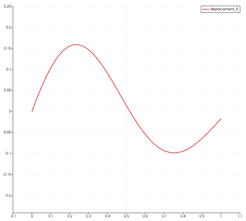
../_images/damped_kv.gif — Displacement field evolution for the Kelvin-Voigt damped wave manufactured solution.¶

Quick Comparison Table¶

Test file	Type	Boundary treatment	Material model	Time setup	Main verification target
`strong_dirichlet.prm`	Static MMS	Strong Dirichlet on 0,1,2,3	Linear elastic, \(\eta=0\)	`Final time = 0.0`	Baseline bulk assembly + strong BC convergence
`weak_dirichlet.prm`	Static MMS	Weak Dirichlet on 0,1,2,3 (penalty 100)	Linear elastic, \(\eta=0\)	`Final time = 0.0`	Weak BC consistency and convergence
`neumann.prm`	Static MMS	Mixed: Dirichlet on 0,2,3 and Neumann on 1	Linear elastic, \(\eta=0\)	`Final time = 0.0`	Traction-term implementation with mixed BCs
`dynamic_purely_elastic.prm`	Dynamic MMS	Weak Dirichlet on 0,1,2,3 (penalty 1000)	Linear elastic, \(\eta=0\)	`Final time = 0.25`, adaptive \(\Delta t\)	Undamped wave propagation in transient solve
`damped_kv_dispersion.prm`	Dynamic MMS	Weak Dirichlet on 0,1,2,3 (penalty 100)	Kelvin-Voigt, \(\eta=0.1\)	`Final time = 1.0`, adaptive \(\Delta t\)	Damping + phase behavior in viscous transient solve

Practical Notes¶

All five files use generated hyper_cube meshes on [0,1]^2.
With inclusions disabled, multiplier blocks are inactive: this is a clean baseline before moving to immersed-coupling tutorials.
Error outputs are written to static_convergence/* or dynamic_convergence/* according to the test.

This is the recommended starting point before enabling reduced-dimensional inclusions in later elasticity tutorials.

Error Tables From The Current Runs (Verbatim)¶

strong_dirichlet.prm¶

cells dofs       u_L2_norm         u_Linfty_norm         u_H1_norm
  50 3.31981741e-02    - 8.13077688e-02    - 5.38879156e-01    -
 162 8.45667720e-03 2.33 2.27197967e-02 2.17 2.69404650e-01 1.18
 578 2.12646951e-03 2.17 5.84286498e-03 2.14 1.34687364e-01 1.09
2178 5.32442180e-04 2.09 1.47114601e-03 2.08 6.73411265e-02 1.05
8450 1.33163499e-04 2.04 3.68443027e-04 2.04 3.36702205e-02 1.02
33282 3.32942254e-05 2.02 9.21518877e-05 2.02 1.68350656e-02 1.01

weak_dirichlet.prm¶

cells dofs       u_L2_norm         u_Linfty_norm         u_H1_norm
  50 3.30005959e-02    - 8.20013285e-02    - 5.39049208e-01    -
 162 8.46483372e-03 2.31 2.27832440e-02 2.18 2.69426674e-01 1.18
 578 2.12811516e-03 2.17 5.84851671e-03 2.14 1.34689122e-01 1.09
2178 5.32634091e-04 2.09 1.47168257e-03 2.08 6.73413277e-02 1.05
8450 1.33184978e-04 2.04 3.68498615e-04 2.04 3.36702578e-02 1.02
33282 3.32967065e-05 2.02 9.21580940e-05 2.02 1.68350730e-02 1.01

neumann.prm¶

cells dofs      u_L2_norm         u_Linfty_norm         u_H1_norm
 18 1.98375493e-01    - 3.14045340e-01    - 1.50171721e+00    -
 50 5.34485579e-02 2.57 1.15380615e-01 1.96 7.45162487e-01 1.37
162 1.37708951e-02 2.31 3.24576646e-02 2.16 3.69915605e-01 1.19
578 3.47449281e-03 2.17 8.45778268e-03 2.11 1.84528306e-01 1.09
2178 8.71006807e-04 2.09 2.15133210e-03 2.06 9.22061056e-02 1.05
8450 2.17937355e-04 2.04 5.42132708e-04 2.03 4.60955985e-02 1.02

dynamic_purely_elastic.prm¶

cells dofs       u_L2_norm         u_Linfty_norm         u_H1_norm      
 578 3.86334173e-02    - 1.07833080e-01    - 1.13104916e+00    - 
2178 1.26657328e-02 1.68 5.42498864e-02 1.04 7.93812513e-01 0.53 
8450 3.40110157e-03 1.94 2.35861056e-02 1.23 4.06259865e-01 0.99 
33282 7.60535360e-04 2.19 6.01771753e-03 1.99 1.58416674e-01 1.37 

damped_kv_dispersion.prm¶

cells dofs       u_L2_norm         u_Linfty_norm         u_H1_norm
 578 6.25099707e-03    - 4.73399423e-02    - 2.02733025e-01    -
2178 1.02433725e-03 2.73 2.39495211e-03 4.50 3.60843614e-02 2.60
8450 3.12743941e-04 1.75 1.77592342e-03 0.44 1.72027908e-02 1.09
33282 7.06583742e-05 2.17 1.37727393e-03 0.37 8.78895167e-03 0.98