Cost of the one-vessel elastodynamics MMS

The one-vessel manufactured solution is small enough for a serial sparse direct solve. Its original runtime came mostly from constructing Jacobian/preconditioner matrices and applying nested iterative solvers. Finite element assembly, lifted pressure evaluation, and output account for a small part of the measured time.

Problem size and measurement scope

Measurements below use the resolved base cube through \(t=0.1\), with the same mesh, quadrature, tolerances, forcing, and output frequency in every solver comparison:

Quantity	Base case
Solid cells	1,024
Displacement unknowns	4,335
Velocity unknowns	4,335
Native flow unknowns, including traces	16
Multiplier unknowns	4
Full coupled Jacobian dimension	8,690
Stored Jacobian entries	1,124,616 initially; 1,124,619 subsequently

The host is an Apple Mac14,6 with 12 CPU cores and 96 GiB RAM, running macOS 26.5.1. These are Release executables from a DebugRelease build, using deal.II 9.8.0-rc1, Trilinos, MetricFlowX 0.1.0, and MPICH 5.0.1. The installed MetricFlowX source commit was not recorded. Each application runs on one MPI rank with one application thread. MPI’s libfabric progress threads can still consume CPU time; summed process CPU time is therefore different from application wall time.

The initial diagnostic run is revision d50da56. A sampling profiler was attached during that run. Compilation was also active on the host, so this run establishes attribution and a baseline observation, not an isolated speed comparison. The controlled comparisons below run sequentially with compilation stopped. Times are local observations, not portable speed guarantees.

Where the original time goes

The initial run took 113.33 s including startup, and 111 s inside the DAE timer. IDA accepted 80 steps, requested five Jacobian setups, and performed 137 linear solves.

Phase	Calls	Wall time	Fraction of DAE time
Jacobian setup, including Schur preconditioner	5	51.0 s	46%
Linear solves	137	57.2 s	52%
Residual evaluation	137	2.34 s	2.1%
Solid spatial assembly	1	0.0301 s	0.027%
Solid body force assembly	139	0.483 s	0.44%
Solid output	4	0.0118 s	0.011%
Native external-pressure residual	10,145	0.590 s	0.53%

The last four rows come from separate component timers. They overlap the adapter phases and must not be added to them.

Two 15-second macOS sample windows explain the expensive phases. Percentages refer only to samples of the application main thread. Inclusive categories overlap; their percentages must not be summed.

Inclusive main-thread stack category	Setup window	Solve window
Jacobian setup	91.5%	0%
Linear solve	8.1%	96.6%
Matrix clone/sum	54.7%	0%
Trilinos row extraction	38.2%	0%
Operator/function copies	23.6%	14.9%
AMG hierarchy construction	0.3%	0%
AMG application	5.3%	62.5%
Epetra sparse matrix-vector products	5.7%	64.9%

The setup window contained 12,080 main-thread samples; the solve window contained 6,334. The first started about 14 s after launch and used a 1 ms sampling interval. The second started about 50 s after launch and used 2 ms. These windows identify active stacks; they do not measure whole-run phase percentages. In particular, the samples implicate matrix copying during setup, not AMG hierarchy construction.

Why a small system can be expensive

Three implementation details amplify the work:

1. A matrix sum previously invoked the first operand’s materializer three times and the other materializers twice. Nested sums multiplied this work. Each operand is now materialized once per sum and retained for the graph and value passes.

2. Repeated calls to Trilinos end(row) construct an accessor that extracts another row. Calling it for every entry adds approximately \(O(Nd^2)\) row-copy work to a scan with \(N\) rows and \(d\) entries per row. Cached row-end iterators and the backend’s native matrix copy reduce these traversals to \(O(\mathrm{nnz})\), apart from graph insertion costs. Distributed copies retain their row/domain partitions and own their data.

3. Structurally absent blocks previously had zero callbacks without deal.II’s is_null_operator flag. Operator products could therefore execute an expensive inverse before multiplying its result by zero. Absent blocks now use dealii::null_operator, and payload erasure preserves the flag.

A separate five-second sample of the refined direct run found another cost in block-to-monolithic conversion: all 3,707 main-thread samples were in that conversion, with 94.69% inside Trilinos end(row) and 5.31% in direct row_length(row) calls. For a completely empty block, both begin(row) and end(row) search forward for a nonempty row. Visiting every empty row therefore costs \(O(N^2)\) even when the row-end iterator is cached. The conversion now checks row length before creating iterators and caches row ends for nonempty rows. These traversals cost approximately \(O(N+\mathrm{nnz})\). The diagnostic refined run was stopped after identifying this issue and is excluded from the completed-run timing comparisons.

The sum optimization retains all materialized operands simultaneously, requiring \(O(\sum_i \mathrm{nnz}_i)\) temporary matrix storage. It trades that storage for fewer copies and materializer calls.

The iterative solve also nests a Schur GMRES inside an outer FGMRES. Before zero-block pruning, an outer preconditioner application with \(k\) Schur actions could invoke approximately \(12+4k\) solid AMG applications and \(2+k\) native flow ILU applications. Residual checks add operator actions. Four multiplier coefficients do not imply four cheap scalar operations: each Schur action can apply inverses on the full solid mesh.

The Schur construction currently creates the participant inverses once for the preconditioner and again for its Schur operator: four solid AMG hierarchies and two flow ILU factorizations per Jacobian setup. This duplication remains; the profile above shows that matrix copying consumed much more setup time than AMG hierarchy construction in this case.

The pressure feedback is evaluated through the native flow residual, including its boundary/interface terms. Creating a new pressure-operator instance requires one native pressure action per global multiplier coefficient to populate its cached matrix. Later materializations of that instance copy the cache. With four coefficients this is small; it can become relevant for a larger network. Increasing axial quadrature improves the lift but does not explain the dominant costs measured here.

MPI diagnostic

A three-second, 2 ms sampling window of rank zero in the optimized two-rank cylinder test contains 1,144 main-thread samples. Linear solves account for 99.4% of them. Inclusive MPI stacks account for 51.5%, distributed vector reinit for 33.9%, AMG applications for 18.0%, and operator/function copies for 16.7%. These categories overlap: vector reinitialization itself can construct maps and enter collective communication.

The test completes with the same 40 accepted IDA steps, 99 right-hand sides, and 4,280 outer FGMRES iterations as the earlier cylinder MPI run. The sample points to repeated vector construction, synchronization, and operator-copy allocation inside the nested solves as remaining costs. Compilation was active during this validation run, so its elapsed time is excluded from the controlled comparisons below. This diagnostic does not establish MPI scaling.

Serial UMFPACK path

subsection MetricFlowX coupled solver
  set Linear solver = umfpack
end

The default remains iterative. The umfpack choice requires exactly one MPI rank and a deal.II installation with UMFPACK. Every IDA Jacobian setup builds \(J=F_y+\alpha F_{\dot y}\) at the callback’s current time and state, materializes the full sparse matrix, and factorizes it with dealii::SparseDirectUMFPACK. All following right-hand sides reuse the factors until the next setup. The direct path bypasses the nested Schur preconditioner. Its timers distinguish Materialize Jacobian, Factorize Jacobian, and Direct backsolve.

Sparse LU costs depend on fill and ordering, not just the original number of entries. For a three-dimensional mesh it should not be assumed to scale linearly in mesh size or to remain memory-efficient after many refinements. This option provides a direct reference solve for small serial verification cases. The matrix-free Jacobian action remains available for checking the true linear residual.

Distributed runs can select Linear solver = mumps when deal.II enables DEAL_II_WITH_MUMPS. This calls dealii::SparseDirectMUMPS directly and reuses each factorization for subsequent right-hand sides. The MMS tutorial provides a parameter file and MPI command. The measurements below use UMFPACK; they do not measure MUMPS performance or parallel scaling.

Controlled comparisons

These runs use the same base input sequentially, without a sampling profiler or concurrent compilation. The original iterative binary includes the new solver selector, set to iterative, and retains the pre-optimization operator implementation at e47b8b5. The optimized binaries include native matrix copies, one materialization per sum operand, zero-block pruning, and the monolithic empty-row fix.

Solver	Jacobian setup	Linear solves	Residuals	Whole process	Maximum resident size
Original iterative	47.9 s	53.1 s	2.22 s	105.99 s	13.07 GiB
Optimized iterative	9.46 s	36.5 s	2.21 s	52.11 s	1.91 GiB
Optimized serial UMFPACK, two runs	5.32–5.59 s	3.65–3.70 s	2.32–2.38 s	13.90–14.96 s	1.12 GiB

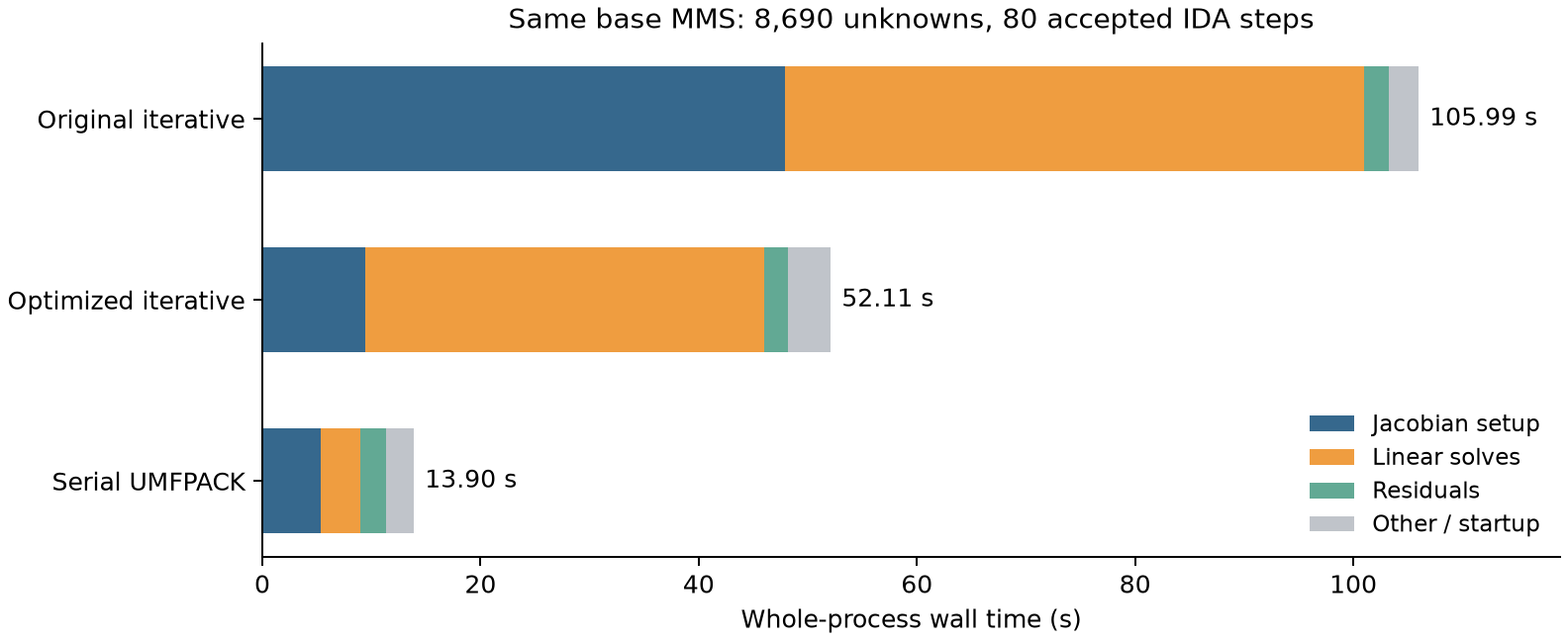
All base runs accept 80 IDA steps, use five Jacobian setups, and solve 137 right-hand sides. Both iterative runs perform exactly 1,668 outer FGMRES iterations, ranging from 5 to 14 per solve. The speedup therefore comes from less work per setup and operator application, with the same outer iteration count. The optimized iterative run takes about half the original time; the direct runs take about one seventh. There is one run of each iterative configuration and two direct runs; these observations do not estimate timing variance across machines or long-term performance.

In the final direct runs, materialization takes 3.20–3.31 s, all five LU factorizations take 0.876–0.954 s, and the 137 backsolves take 3.65–3.70 s. Materialization and factorization are included in Jacobian setup, and backsolves are included in linear solves. These nested timers must not be added a second time. Backsolve time includes conversion between the execution block vectors and serial vectors. Maximum resident size is macOS /usr/bin/time -l’s process statistic, converted from bytes to GiB; it is not the sparse factors’ storage alone.

The optimized iterative fields are identical to the original exported fields. Direct-solve differences at final time are at Float32 output precision: relative nodal differences are below \(7\times10^{-9}\) for solid displacement and velocity, below \(4\times10^{-8}\) for the multiplier, and below \(2\times10^{-14}\) for flow velocity. Exported area values are identical. The solver changes preserve the coarse mesh’s discretization errors; the MMS tutorial reports those errors separately.

The refined cube has 8,192 solid cells, 29,403 unknowns per solid field, 32 native flow unknowns, and eight multiplier unknowns: 58,846 unknowns in total. The complete refined serial UMFPACK run reaches \(t=0.1\) in 120.07 s, with 69 accepted steps, five Jacobian setups, and 77 right-hand sides. Its Jacobian stores 8,471,852 entries initially and 8,471,861 subsequently. Maximum resident size is 7.37 GiB.

Refined serial direct phase	Wall time
Jacobian materialization	18.2 s
LU factorization	38.7 s
Backsolves, including vector conversion	40.0 s
Residual evaluation	6.23 s

Factorization and backsolves now dominate. The unknown count grows by a factor of 6.77 and stored entries by 7.53; factorization time grows by about 44 relative to the second base run. This is consistent with the cost of sparse LU fill, but two meshes do not establish an asymptotic scaling rate. The refined displacement error (16.84%), multiplier error (24.45%), inlet flux (\(4.4367093\times10^{-6}\)), and relative volume defect (0.04997%) reproduce the earlier iterative measurements. The earlier refined iterative run used two ranks, so its 465.83 s is not a same-rank solver comparison.

Reproduce the measurements

Use the build-tree parameter files, after configuring and building the target:

cmake --build /path/to/build --target metric_flow_x_elastodynamics -j2
cd /path/to/build
/usr/bin/time -l ./metric_flow_x_elastodynamics \
  tutorials/metric_flow_x_elastodynamics/mms_cube.prm > iterative.log 2>&1

For a direct run, create an override outside the source tree:

include /absolute/build/path/tutorials/metric_flow_x_elastodynamics/mms_cube.prm
subsection MetricFlowX coupled solver
  set Linear solver = umfpack
end
subsection Elastodynamics
  set Output directory = /absolute/results/direct/solid
end
subsection MetricFlowSystem<1, 3>
  set Output directory = /absolute/results/direct/flow
end

Give each comparison its own output directory and retain the complete logs. On macOS, sample an active process from another terminal:

sample PID 15 1 -mayDie -fullPaths -file setup.sample.txt
sample PID 15 2 -mayDie -fullPaths -file solve.sample.txt

Choose windows from the actual runtime. A short optimized run may finish before a 15-second sample completes. Read the main-thread call tree separately from MPI progress threads and profiler symbolication time. Use full application timers for phase totals, and sampling stacks to explain those totals.