One vessel in a cube: a manufactured solution

This example prescribes a nonzero, time-dependent radial displacement, vessel area, axial velocity, and pressure-jump multiplier. A continuous, piecewise solid displacement supplies the stress jump needed to balance the multiplier. The inlet supplies the increase in vessel volume; physical continuity has no distributed mass source.

The inputs exercise all five residual rows of metric_flow_x_elastodynamics. Displacement compatibility is imposed in the multiplier row, while its traction acts in solid momentum. Continuity has no multiplier reaction. The flow receives the external pressure \(p_{\mathrm{ext}}=-\lambda\) through native volume, face, boundary, and junction equations.

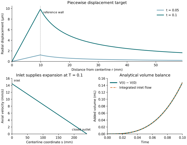
This figure shows the analytical target.

Configure and run

The parameter templates are in tutorials/metric_flow_x_elastodynamics/:

Template	Solid cells	Centerline cells	Purpose
mms_cube.prm.in	\(4\times16\times16\)	2	Single-rank MMS
mms_cube_refined.prm.in	\(8\times32\times32\)	4	Refine both meshes
mms_cube_mpi.prm.in	\(4\times16\times16\)	2	Separate output directories for MPI
mms_cube_neumann.prm.in	\(4\times16\times16\)	2	Exact Neumann traction
mms_cube_neumann_refined.prm.in	\(8\times32\times32\)	4	Exact Neumann traction on refined meshes

All cases use degree-one elements, an automatically matched multiplier space, and the same analytical target. Centerline cells have twice the length of solid cells in the axial direction: \(h_\gamma=2h_x=L/2\) in the base case and \(L/4\) in the refined case. The solid cells have \(h_x=4h_y=4h_z\). Both meshes are refined together.

This ratio keeps the DG1 multiplier mesh coarser than the continuous Q1 solid trace. On this Cartesian tensor-product mesh, four solid axial cells provide five continuous axial modes. Four DG1 multiplier cells would introduce eight coefficients, so the mechanical pairing alone could not distinguish all multiplier modes. Two DG1 cells introduce four coefficients.

The wall lift uses composite Gauss quadrature: two repetitions of four points per centerline cell. Each repetition spans one solid axial cell, giving four axial quadrature sections per solid cell, or 16 sections in the base case and 32 in the refined case. Three points on a single vessel cell sample only three sections across four solid cells and can produce artificial axial variation even though the target solid displacement is independent of \(x\). Check quadrature sensitivity separately from mesh refinement. The axial settings are:

subsection MetricFlowX vessel wall lift
  subsection Representative quadrature
    set Type = gauss
    set Number of points = 4
    set Number of repetitions = 2
  end
end

The cross-section refinement level is two in the base and MPI inputs and three in the refined input, so refinement also improves wall geometry.

The target area is constant in space and the target velocity is linear, so degree one represents both exactly on either centerline mesh. Both cases use single_vessel_centered.vtk, which contains one coarse cell. The base and MPI inputs set Number of global refinement = 1; the refined input sets it to 2. These produce two and four centerline cells, respectively.

The flow is constructed before its observing Domain. During flow setup, Domain copies the coarse mesh with its native vessel and terminal ids, imports all VTK properties, transfers them during refinement, and partitions the final mesh. The lift uses flow_domain.field("a0"); it does not reread the VTK after refinement. This requires the setup(mesh_initializer) overload from MetricFlowX PR #35.

Configure with a compatible MetricFlowX package and deal.II with SUNDIALS and VTK enabled. For example, from the repository root:

cmake -S . -B build-mms -DCMAKE_BUILD_TYPE=Release \
  -DMetricFlowX_DIR=/path/to/metric-flow-x/lib/cmake/MetricFlowX
cmake --build build-mms --target metric_flow_x_elastodynamics -j2

Require MetricFlowX support enabled in the configuration output. Pass DEAL_II_DIR as well if deal.II is not already discoverable. A Debug build uses the target and executable metric_flow_x_elastodynamics_debug.

CMake generates the runtime inputs, including the absolute include path in the refined and MPI cases. Run the generated .prm files from the build directory so that the application’s last_used_parameters.prm also stays there:

cd build-mms
./metric_flow_x_elastodynamics \
  tutorials/metric_flow_x_elastodynamics/mms_cube.prm
./metric_flow_x_elastodynamics \
  tutorials/metric_flow_x_elastodynamics/mms_cube_refined.prm
mpirun -np 2 ./metric_flow_x_elastodynamics \
  tutorials/metric_flow_x_elastodynamics/mms_cube_mpi.prm

The default inputs prescribe exact time-dependent Dirichlet data. To run the same target with exact Neumann traction, use:

./metric_flow_x_elastodynamics \
  tutorials/metric_flow_x_elastodynamics/mms_cube_neumann.prm
mpirun -np 2 ./metric_flow_x_elastodynamics \
  tutorials/metric_flow_x_elastodynamics/mms_cube_neumann_refined.prm

The Neumann variants write to metric-flow-x-mms-cube-neumann and metric-flow-x-mms-cube-neumann-refined below test_output/, so they can be compared with the Dirichlet runs without replacing their output.

Reconfigure after changing a template. These inputs select one spatial solve each; Number of refinement cycles does not make this coupled executable perform a convergence study. Configure the integration interval and adaptive IDA controls in MetricFlowSystem<1, 3>/IDA parameters, as in the two-way example. The coupled application does not declare a Fixed step section.

For a serial run, select a sparse direct solve with:

subsection MetricFlowSystem<1, 3>
  subsection IDA parameters
    subsection Linear solver
      set Type = umfpack
    end
  end
end

The default is iterative. This selects the full coupled solve; the native MetricFlowX Use direct solver parameter controls its own local solver. The umfpack option requires a deal.II build with UMFPACK and exactly one MPI rank. Each IDA Jacobian setup materializes the full coupled matrix \(J=F_y+\alpha F_{\dot y}\) at the current time and state and factorizes it. Subsequent linear solves reuse that factorization until IDA requests another setup. This bypasses the iterative Schur preconditioner. The timer summary separates matrix materialization, factorization, and direct backsolves. Materialization uses the existing sparse block assembly; a native pressure block that has no assembled matrix is recovered from its operator columns. This path is intended for small serial verification problems. See the cost analysis and profiling report for measured setup and solve costs.

For a distributed direct solve, select Linear solver/Type = mumps. This uses dealii::SparseDirectMUMPS directly and requires DEAL_II_WITH_MUMPS in the deal.II configuration. Run the generated example with:

mpirun -np 2 ./metric_flow_x_elastodynamics \
  tutorials/metric_flow_x_elastodynamics/mms_cube_mumps.prm

MUMPS also works on one rank. It uses the same current Jacobian and factor reuse policy as UMFPACK. The matrix and right-hand side retain their native ownership; the solution is redistributed from contiguous MUMPS output to the coupled fields. The total number of coupled unknowns must be at least the number of MPI ranks. This option does not use the PETSc or Trilinos direct solver interfaces.

The local macOS installation (deal.II 9.8.0-rc1, MUMPS 5.9.0) fails in DMUMPS_SCATTER_DIST_RHS on the coupled application, after successful factorization, in serial and MPI. Distributed analytical checks also fail in that installation. A similar failure is tracked in deal.II issue #19513. The Linux deal.II 9.7.1 installation passes the serial and MPI analytical checks in Debug and Release. These results do not establish that every MUMPS-enabled installation can run the application.

Geometry and coefficients

The solid fills the cube \(\Omega=[-\ell,\ell]^3\), with \(\ell=0.120685\). The straight centerline is \(\gamma=\{(x,0,0):-\ell\le x\le\ell\}\), of length \(L=2\ell=0.24137\). The data/metric_flow_x/single_vessel_centered.vtk.in input supplies

\[ A_0=a_d=3.0605\times10^{-4},\qquad R_0=\sqrt{A_0/\pi}\simeq0.00987009324508. \]

The fictitious solid inside the vessel is part of the cube. The immersed reference wall is \(\Gamma_0=\{r=R_0\}\), where \(r=\sqrt{y^2+z^2}\). Its radius is fixed in the lift; the current area enters the displacement increment.

The solid density and Lamé coefficients are \(\rho_s=\lambda_s=\mu_s=1\), with zero damping. These are verification coefficients. Flow density is \(1060\), viscosity is zero, and the existing VTK tube-law properties are retained. The numerical time interval is \(0\le t\le T=0.1\).

Piecewise solid solution

Let \(g(t)=t^3\) and define the spatial vector

\[\begin{split} w(x,y,z)= \begin{cases} (0,y,z), & r\le R_0,\\[2pt] \displaystyle\frac{R_0^2}{r^2}(0,y,z), & r>R_0. \end{cases} \end{split}\]

The target displacement, velocity, and body force are

\[ u^\star=t^3w,\qquad v^\star=3t^2w,\qquad f^\star=6\rho_s t\,w. \]

The displacement is continuous at \(r=R_0\) and regular at the centerline. Its radial derivative jumps at the wall. Away from the wall, both \(r\) and \(R_0^2/r\) solve the radial homogeneous elasticity equation, so \(\operatorname{div}\sigma(u^\star)=0\) in each subdomain. Thus the body force above supplies the acceleration without a volume approximation to a surface force.

For

\[ \sigma(u)=2\mu_s\varepsilon(u)+\lambda_s\operatorname{div}(u)I, \]

the radial stresses at the interface are

\[ \sigma_{rr}^{\mathrm{in}}=2(\lambda_s+\mu_s)g,\qquad \sigma_{rr}^{\mathrm{out}}=-2\mu_s g. \]

With \(n\) directed from the centerline toward the surrounding solid, the jump is \([\sigma n]=(\sigma^{\mathrm{in}}-\sigma^{\mathrm{out}})n\). The momentum balance

\[ (\rho_s\dot v,\phi)_\Omega+ (\sigma(u),\varepsilon(\phi))_\Omega- (f,\phi)_\Omega+ \int_{\Gamma_0}\lambda\,n\cdot\phi\,d\Gamma- \int_{\partial\Omega}\tau\cdot\phi\,dS=0 \]

therefore requires

\[ \lambda^\star=-2(\lambda_s+2\mu_s)g=-6t^3. \]

This is the scalar pressure-jump multiplier. Its negative sign balances the outward displacement under the positive solid-reaction convention.

All cube faces have boundary id zero. Prescribe the exact displacement \(u^\star=t^3w\) and velocity \(v^\star=3t^2w\) on every face, including the vessel end planes. Both initial fields are zero. The initial acceleration and multiplier are also zero, matching the application’s initialization. The parameter expressions use \(R_0^2/\max(y^2+z^2,R_0^2)\) to encode both branches without division by zero.

The elastodynamics contributor updates boundary values before evaluating any residual or Jacobian term. The displacement weak term automatically refreshes the contribution of prescribed values at each candidate time while retaining the coupling matrix. Constraint indices and master entries must remain fixed during the solve.

The Neumann variants instead prescribe the exact outer traction \(\tau^\star=\sigma(u^\star)n_\Omega\) on every face. They select Neumann boundary id zero and leave the Dirichlet ids empty. For \(r<R_0\), the stress matrix is \(t^3\operatorname{diag}(2,4,4)\). For \(r>R_0\), its nonzero components are

\[ \sigma_{yy}=\frac{2t^3R_0^2(z^2-y^2)}{r^4},\qquad \sigma_{zz}=-\sigma_{yy},\qquad \sigma_{yz}=\sigma_{zy}=-\frac{4t^3R_0^2yz}{r^4}. \]

The boundary expression multiplies this matrix by the appropriate cube-face normal, using a coordinate tolerance of \(10^{-10}\) to identify faces and regularizing denominators where the numerator is zero. The transient mass operator and zero initial displacement and velocity fix the rigid-body motion.

Area and volume supplied by the inlet

On the reference wall, \(u^\star\cdot n=R_0g\). The area-to-radius relation therefore gives the spatially uniform target

\[ A^\star(t)=A_0(1+t^3)^2,\qquad \dot A^\star(t)=6A_0t^2(1+t^3). \]

Let \(s=x+\ell\in[0,L]\). Use

\[ Q^\star(s,t)=(L-s)\dot A^\star(t),\qquad U^\star(x,t)=(\ell-x)\frac{6t^2}{1+t^3}. \]

These fields satisfy source-free continuity pointwise:

\[ \partial_t A^\star+\partial_s(A^\star U^\star)=0. \]

At the endpoints,

\[ Q_{\mathrm{in}}^\star=L\dot A^\star,\qquad Q_{\mathrm{out}}^\star=0,\qquad \frac{d}{dt}(LA^\star)=Q_{\mathrm{in}}^\star-Q_{\mathrm{out}}^\star. \]

The inlet function is this nonzero, time-dependent volumetric flow rate. The outlet uses Reflection with Rt = 1. The native characteristic equations then impose zero outlet velocity. Zero outlet flux is compatible with expansion because the inlet supplies all of the added volume. Setting both endpoint fluxes to zero would require a distributed mass source.

For this target, the tube-law pressure is uniform along the vessel. With zero friction, the native momentum equation uses \(p=p_{\mathrm{tube}}(A)-\lambda\):

\[ \partial_t U+U\partial_s U+\rho_f^{-1}\partial_s p=S_U. \]

Consequently the two RHS expressions are

\[ S_A=0,\qquad S_U=(\ell-x)\frac{12t-42t^4}{(1+t^3)^2}. \]

Both tube-law pressure and multiplier are spatially uniform for this target. Their pressure gradient vanishes. Native pressure contributions at faces and boundaries must still be assembled to cancel the volume contribution.

Residual rows and their forcing

With \(C(u,A)=B^Tu-P_h(A)\), the assembled rows are

\[\begin{split} \begin{aligned} F_u &= M(\dot u-v),\\ F_v &= M\dot v+Ku-f+B\lambda,\\ F_A &= F_A^{\mathrm{native}},\\ F_U &= F_U^{\mathrm{native}}+F_U^{\mathrm{pressure}}(-\lambda),\\ F_\lambda &= B^Tu-P_h(A). \end{aligned} \end{split}\]

Here \(f\) includes body force and outer Neumann traction. Native algebraic trace rows also receive their pressure contributions. The displacement constraint produces a traction through its derivative with respect to \(u\). Introducing \(v=\dot u\) places that traction in the momentum residual, which is registered under \(v\). It does not replace displacement compatibility with a velocity constraint.

The prescribed RHS is zero in the kinematic, continuity, and multiplier rows. The momentum RHS contains \(6t\,w\) and the exact outer traction; the flow velocity RHS is \(S_U\) above. No source compensates for an erroneous multiplier reaction in continuity. In particular, \(-DP_h(A)\) belongs to the multiplier row’s area derivative, and \(B\) belongs to the momentum row’s multiplier derivative.

The application shows all coupling terms together: two weak terms for compatibility, one for momentum traction, and the native pressure residual with its multiplier derivative. The generic symmetric make_constraint(...) remains appropriate when a constraint’s transpose reactions belong to the same participant residual rows.

The pressure derivative uses native assembly for its forward action. A transpose or explicit matrix request collectively probes the multiplier basis; this costs one native assembly per global coefficient. Pressure evaluation uses the native CellId to preserve DG traces and exchanges ghost coefficients. Pressure coefficients are differentiated at the candidate flow state. The Jacobian omits derivatives of HLL characteristic-speed weights, following the native flow Jacobian’s frozen-speed approximation. The application also enables one off-diagonal primal correction in the Schur approximation, retaining the multiplier-to-velocity-to-displacement path. Elimination and recovery use the same corrected primal inverse.

Inspect the solution

Outputs are below the build-tree test_output/ directory, in separate metric-flow-x-mms-cube-resolved, metric-flow-x-mms-cube-refined-resolved, and metric-flow-x-mms-cube-mpi-resolved directories. Each contains solid.pvd, flow.pvd, and the multiplier series pressure_jump.pvd in the same directory. Flow output contains area, velocity, A_hat, U_hat, and pressure. CTest adds a configuration and case prefix, such as Release/metric-MMS-Serial/, before these output directories.

At the final target time \(T=0.1\):

Quantity	Analytical target
Area \(A^\star\)	\(3.0666240605\times10^{-4}\)
Radial wall increment \(R_0T^3\)	\(9.87009324508\times10^{-6}\)
Pressure jump \(\lambda^\star\)	\(-0.006\)
Inlet velocity \(U^\star(-\ell,T)\)	\(0.0144677322677\)
Inlet flow \(Q_{\mathrm{in}}^\star(T)\)	\(4.43670958731\times10^{-6}\)
Outlet flow \(Q_{\mathrm{out}}^\star(T)\)	\(0\)

In ParaView, compare the solid radial displacement along a transverse line with \(t^3r\) inside and \(t^3R_0^2/r\) outside. Compare the centerline area with \(A_0(1+t^3)^2\), axial velocity with \((\ell-x)6t^2/(1+t^3)\), and pressure_jump with \(-6t^3\). Use the accepted physical time, not a file index.

All three output series use the accepted simulation times and contain the initial state once.

Check the integrated volume balance independently:

\[ V_h(t)=\int_\gamma A_h\,ds,\qquad \frac{dV_h}{dt}\mathrel{?}=Q_{\mathrm{in},h}-Q_{\mathrm{out},h}. \]

For the target, the increase is \(V^\star(t)-V^\star(0)=LA_0[(1+t^3)^2-1]\). A centered difference between outputs only approximates the volume derivative; distinguish that error from a conservation defect.

The application does not call either Problem’s error routine or produce coupled error tables. The Exact solution entries store the target formulas; they do not activate error computation. Compare exported fields externally. Do not claim convergence to this target from successful solver exits or from agreement between serial and MPI runs. The piecewise stress field, unfitted solid mesh, cross-section geometry, and time error must also be considered when interpreting differences between the two meshes.

Local verification results

The measurements and plots below used exact Neumann traction on all cube faces. They correspond to the retained Neumann variants and do not measure the time-dependent Dirichlet inputs above.

Runs on 2026-10-22 used deal.II 9.8.0-rc1, MPICH 5.0.1, and an installed MetricFlowX package reporting version 0.1.0 with both build variants. The installed package’s source revision was not recorded. The corrected base case reached \(T=0.1\) in 80 accepted IDA steps; the refined case took 69. The base case ran in serial and on two ranks in Debug and Release. The refined measurement used Release on two ranks.

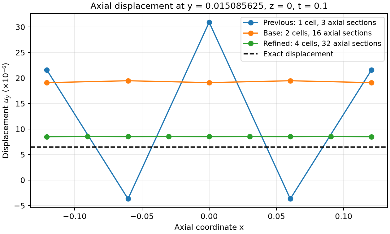
The plot compares \(u_y\) at \(y=0.015085625\), \(z=0\), \(t=0.1\). The previous single-cell vessel used three axial integration sections; the corrected base case uses two vessel cells and 16 sections. The background mesh is \(4\times16\times16\) in both cases. The refined curve uses the \(8\times32\times32\) solid, four vessel cells, and 32 axial sections. Matching the mesh scales and using composite quadrature removes the large axial oscillation on this line. The corrected base value still exceeds the exact displacement by about a factor of three; the refined curve is much closer to the target. A smoother contour alone is not evidence of an accurate MMS solution.

The relative nodal axial variation decreases from \(0.655\) to \(0.125\) in the corrected base case and to \(0.0171\) in the refined case. For this diagnostic, group nodes with the same \((y,z)\), subtract their mean displacement over all axial nodes, and divide the Euclidean norm of these differences by the Euclidean norm of the displacement. Count each geometric node once. This diagnostic measures axial variation; it is not an \(L^2\) error against the target.

Quantity at \(T=0.1\)	Corrected base mesh	Refined mesh
\(|u_h-u^\star|_{L^2(\Omega)}\)	\(1.8260\times10^{-7}\)	\(3.4130\times10^{-8}\)
Relative \(L^2\) displacement error	\(0.8987\)	\(0.1684\)
\(|v_h-v^\star|_{L^2(\Omega)}\)	\(6.1092\times10^{-6}\)	\(1.1318\times10^{-6}\)
Relative \(L^2\) solid velocity error	\(1.0022\)	\(0.1861\)
Relative \(L^2\) area error	\(7.5552\times10^{-7}\)	\(1.0055\times10^{-6}\)
\(|U_h-U^\star|_{L^2(\gamma)}\)	\(2.5987\times10^{-9}\)	\(4.2567\times10^{-9}\)
Relative \(L^2\) multiplier error	\(1.3619\)	\(0.2445\)
Mean multiplier	\(-0.01417113\)	\(-0.00746724\)
Added volume	\(1.4787187\times10^{-7}\)	\(1.4789031\times10^{-7}\)
Volume defect / prescribed influx	\(0.03749\%\)	\(0.04997\%\)

The exact multiplier is \(-0.006\), and the integrated prescribed influx is \(1.478164482885\times10^{-7}\). The coarse solid mesh remains inaccurate: the displacement and multiplier errors are larger than the earlier underintegrated results. The refined solid reduces both errors substantially, but the two meshes and two wall geometries do not establish an asymptotic convergence rate. The vessel diameter spans only about 1.31 transverse solid cells in the base case and 2.62 in the refined case. Resolve the transverse piecewise displacement and wall geometry further, and reduce the time tolerances before drawing conclusions about convergence. The old underintegrated error table does not validate the corrected inputs.

The measurements integrate the exported Float32 fields. Solid errors use three-point tensor-product Gauss quadrature on each cube cell, comparing interpolated displacement and velocity with the piecewise analytical fields. Centerline errors, means, and volumes use two-point Gauss quadrature on the exported linear fields. Relative errors divide by the exact field’s \(L^2\) norm. The volume defect is the final area integral minus its initial value and the exact integrated inlet flow. Physical times come from the multiplier series, because the native flow writer’s clock remains at zero.

CTest runs both boundary variants in Debug and Release, in serial and on two ranks. Its application regressions use a \(4\times8\times8\) solid mesh, a coarser cross-section quadrature and final time \(T=0.02\), with outputs at \(0\), \(0.01\) and \(0.02\). They retain the manufactured forcing, solver tolerances and both flow cells, and must finish within 115 seconds. The tutorial templates above retain their resolved meshes and \(T=0.1\) accuracy runs. These application tests check that integration finishes. Separate integration tests check multiplier row placement, unchanged continuity, the nonlinear Jacobian action by finite differences on the single-cell fixture, nonzero corrections for tiny right-hand sides, and rejection of failed IDA steps in Release. Field errors and volume balance provide the analytical comparisons reported above.