This second deal.II laboratory focuses on the mesh itself: its geometric entities, topological relations and representation in software. Start by examining a simple file, then see how deal.II manages the bookkeeping behind an object-oriented interface.
Guiding question: If you had to represent a mesh in a computer program, what information would you need to store?
Learning objectives
By the end of the lesson you should be able to:
distinguish vertices, cells, faces, coordinates and connectivity;
read a small legacy ASCII VTK
UNSTRUCTURED_GRID;explain why two cells share a face even when it is not listed separately;
construct a
Triangulation<2>withGridGenerator;iterate over active cells, vertices and faces via object methods;
count boundary faces without reconstructing a neighbour table;
export a mesh with
GridOutand inspect it in ParaView;explain why a curved geometry may require a
Manifoldwhen refining.
1. What is a mesh?
Consider the domain , divided into two quadrilaterals. Number the six vertices like this:
3 -------- 4 -------- 5
|          |          |
|  cell 0  |  cell 1  |
|          |          |
0 -------- 1 -------- 2
Where would you store vertex coordinates? How would you describe which vertices belong to each cell? How would you find a neighbouring cell or decide that a face is on the boundary?
This mesh has 6 vertices, 2 quadrilateral cells, and 7 distinct faces: 6 on the boundary and 1 shared. If you walk around both cells, however, you visit 8 cell-face incidences. The internal face belongs to both cells. The distinction between a geometric entity and its incidences is fundamental.
A MATLAB-style representation might store one array of vertex coordinates, another array of cell-to-vertex connectivity, and perhaps arrays for faces and adjacency. All of this data must exist in some form; the question is whether application programmers must handle it explicitly.
2. A complete VTK file
Open the repository file
labs/lab-02/data/two-quads.vtk
with a text editor. Here is the complete file:
# vtk DataFile Version 3.0
Two adjacent quadrilaterals
ASCII
DATASET UNSTRUCTURED_GRID
POINTS 6 float
0 0 0
1 0 0
2 0 0
0 1 0
1 1 0
2 1 0
CELLS 2 10
4 0 1 4 3
4 1 2 5 4
CELL_TYPES 2
9
9
Interpretation:
POINTS 6 floatgives the coordinates of six points. VTK uses three coordinates here; the third is zero for this planar mesh.CELLS 2 10gives two connectivity records containing ten integers in total: each record starts with4and then lists four zero-based point indices.CELL_TYPES 2gives one type code per cell. Type 9 denotes a VTK quad.
The first cell is (0,1,4,3) and the second is (1,2,5,4). Both refer to
vertices 1 and 4: they therefore share that edge. No explicit table of
faces is required in this file.
Open the file in ParaView, press Apply, and use Surface With Edges or Wireframe to identify the two cells.
Exercise A. Change the coordinates of vertex 4 in the text file and reload it. Which cells are affected? Restore the original file.
Exercise B. Duplicate both vertices 1 and 4 with new indices but identical coordinates, and make only the second cell use the copies. The picture can remain unchanged, although the cells no longer share point identities. Explain why geometry and connectivity are different. This demonstrates a topological distinction; an application may still regard coincident but disconnected cells as an invalid computational mesh.
Reference: VTK legacy file format.
3. From arrays to a mesh object
Open labs/lab-02/lab-02.cc.
The code creates an equivalent mesh:
Triangulation<2> tria;

GridGenerator::subdivided_hyper_rectangle(
  tria,
  std::vector<unsigned int>{2, 1},
  Point<2>(0., 0.),
  Point<2>(2., 1.));
Identify the C++ concepts:
Triangulation<2>is a class template, andtriais an object.GridGeneratoris a namespace providing mesh generation functions.Point<2>represents a point in two dimensions.The cells are quadrilaterals. In deal.II, the word triangulation refers to a mesh; it does not imply that every cell is a triangle.
Object-oriented abstraction is not the absence of adjacency information. It is the ability to ask the mesh for geometrical/topological properties without knowing how the library stores and maintains them.
4. Iterate over cells, vertices and faces
Here is a loop over the active cells of the triangulation:
for (const auto &cell : tria.active_cell_iterators())
std::cout << cell->center() << '\n';The distinction between active and parent cells is covered in a later lab.
For the initial unrefined mesh, all cells are active. The expression
cell->center() is a method call through an iterator-like cell handle.
Next, inspect cell vertices:
for (const auto &cell : tria.active_cell_iterators())
  for (unsigned int v = 0; v < cell->n_vertices(); ++v)
    std::cout << "Vertex " << v << ": " << cell->vertex(v) << '\n';
Notice that a shared vertex is printed once from each adjacent cell,
although tria.n_vertices() counts distinct vertices.
Finally, traverse cell faces:
for (const auto &cell : tria.active_cell_iterators())
  for (unsigned int f = 0; f < cell->n_faces(); ++f)
    {
      const auto face = cell->face(f);
      if (face->at_boundary())
        std::cout << "Boundary id: " << face->boundary_id() << '\n';
    }
An API call such as face->at_boundary() replaces the need to build a
neighbour table in application code. It expresses the mathematical
question directly.
Exercise 1. Write a function taking const Triangulation<2> &
which returns the number of boundary faces. Predict the answer before
executing the program.
Exercise 2. Add up cell->n_faces() for every active cell. Why is this
number 8 while the number of distinct faces is 7?
Exercise 3. Change the subdivisions from {2,1} to {3,2}.
Predict the number of active cells, vertices and boundary faces and
compare the result. Why does your boundary-counting function need no
modification?
Initial reference values: 2 active cells; 6 vertices; 6 boundary faces; 1 shared interior face.
5. Build and export the mesh
Run the following from the repository root, inside the provided devcontainer (deal.II 9.7.1) or a compatible installation:
cmake -S . -B build -DCMAKE_BUILD_TYPE=Release
cmake --build build --target lab-02 --parallel 2
./build/bin/lab-02 rectangle
The reference program saves output/rectangle.vtk through GridOut:
GridOut grid_out;
std::ofstream output("output/rectangle.vtk");
grid_out.write_vtk(tria, output);
The actual implementation uses a helper to create the output directory
and check for errors. In ParaView, compare the output with the handwritten
two-quads.vtk file.
The geometrical mesh is equivalent, but VTK point numbering, record ordering and metadata need not be identical. deal.II can export material and manifold identifiers alongside the cells. See GridOut (deal.II 9.7).
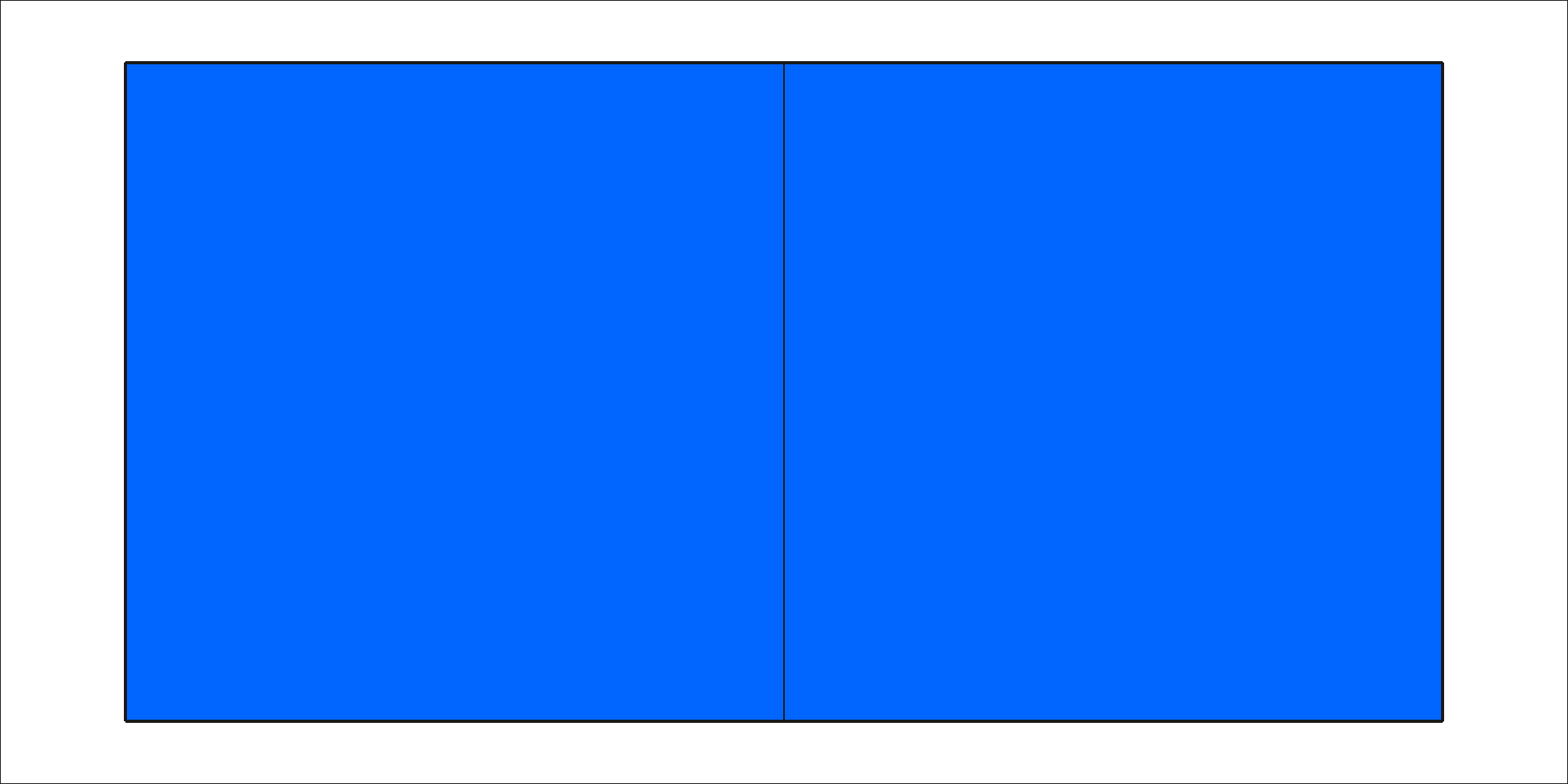
Figure 1:Two adjacent quadrilaterals generated by the course tests with GridOut.
6. Geometry, curved boundaries and manifolds
So far, coordinates and connectivity have been treated separately. A further question arises when refining a curved domain: Where should the new vertices be placed?
Imagine an annulus. The midpoint of a straight chord between two points on a circle does not lie on that circle. Inserting new vertices at straight-line midpoints makes the refinement follow a polygonal approximation rather than the intended curved boundary.
The Manifold interface provides geometrical information to deal.II’s
refinement machinery without putting circle-specific formulas into the
application’s traversal code.
Try both modes of the example:
./build/bin/lab-02 shell-flat
./build/bin/lab-02 shell-curved
Both start with GridGenerator::hyper_shell and an identical coarse annular
mesh. The generator attaches a SphericalManifold by default. In
shell-flat, the call to tria.reset_all_manifolds() disables that curved
description before refine_global(2). In shell-curved, the attached
spherical manifold remains available when new vertices are inserted.
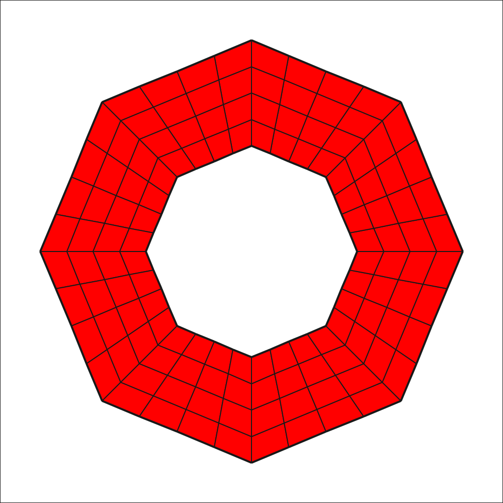
Figure 2:With flat geometry, new boundary points lie on the polygonal chords.
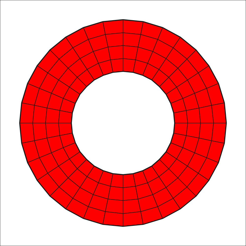
Figure 3:With the spherical manifold, refinement respects the circular geometry.
Open output/shell-flat.vtk and output/shell-curved.vtk in ParaView,
choose the wireframe representation, and zoom in on the two circular
boundaries. Examine the positions of the newly created vertices.
Two IDs have different roles. A boundary_id identifies a part of
the boundary for later use, for example when specifying boundary
conditions. A manifold_id identifies the geometric description used
for operations such as refinement. They are not interchangeable.
Mathematical details of manifolds, hierarchical mesh storage, and higher-order finite element mappings are outside the scope of this lab. The key idea is that topology and geometry are separate responsibilities. For more see deal.II step-1.
7. Discussion and final exercise
Test your boundary-face-counting function on the two-quadrilateral mesh, a larger subdivided rectangle, and one of the annular meshes.
Explain aloud: Which queries concern topology? Which concern geometry? How would you reconstruct the same information using only arrays? Why does your function work for different meshes without modification? And why is extra geometrical information needed when refining curved domains?
Takeaway
A triangulation is a collection of geometric entities with incidence relations. A VTK file makes coordinates and cell connectivity visible. deal.II encapsulates the representation behind a stable, object-oriented interface. A manifold is a further abstraction that informs geometric operations without exposing their internal implementation.
Next laboratory: finite element spaces and degrees of freedom.