This first laboratory is a practical introduction to the tools that we will use throughout the course. We will synchronize the course material with Git, edit a C++ source file in VS Code, configure and build it with CMake, generate a small CSV data set, and inspect the result in ParaView.
The example deliberately does not use deal.II yet. Before using a finite element library, it is useful to understand the complete workflow with a small, self-contained program.
Learning objectives
By the end of this laboratory, you should be able to:
update a local copy of the course material with
git pull;open a project folder and edit source files in VS Code;
read a minimal
CMakeLists.txtfile;configure and build an out-of-source C++ project;
recognize a class template such as
Point<dim, Number>;generate a human-readable CSV file from a C++ program;
load a CSV file in ParaView and turn its rows into points.
construct a simple 2D contour pipeline from CSV data;
extend the program to three dimensions and experiment with 3D isosurfaces and opacity.
The course repository is maintained by the lecturer. You do not need to push your laboratory work to the lecturer’s repository. Git is used here primarily to keep your local copy of the lectures and laboratories synchronized.
1. Synchronizing the course material with Git
Clone the repository once, before the first laboratory:
git clone https://github.com/luca-heltai/nmpde.git
cd nmpde
Before every subsequent lecture or laboratory, update the local copy:
git pull --ff-only
git status
The --ff-only option makes the intended workflow explicit: the course copy
should follow the lecturer’s repository without creating a merge commit. If
you have modified a file inside the course copy, save that work elsewhere
before pulling or ask the lecturer for help.
A convenient arrangement is to keep two directories:
nmpde/          # the read-only course copy, updated with git pull
my-labs/        # your personal solutions and experiments
For this laboratory, the reference source is in
labs/lab-01/lab-01.cc. You may copy it to a personal directory before
modifying it. Local commits and a personal repository are optional; neither
is a contribution to the lecturer’s repository.
The official Git documentation on creating a repository and the VS Code source-control overview are useful references.
2. Opening the project in VS Code
Open the repository folder, rather than only opening a single source file:
code .If the code command is not available, open the folder using File → Open
Folder. The integrated terminal should start in the project directory.
The most useful areas for this course are:
the Explorer, for navigating files and folders;
the editor, for changing source files;
the Source Control view, for seeing local changes;
the integrated terminal, for running Git, CMake, and executables;
the Problems view, for reading compiler diagnostics.
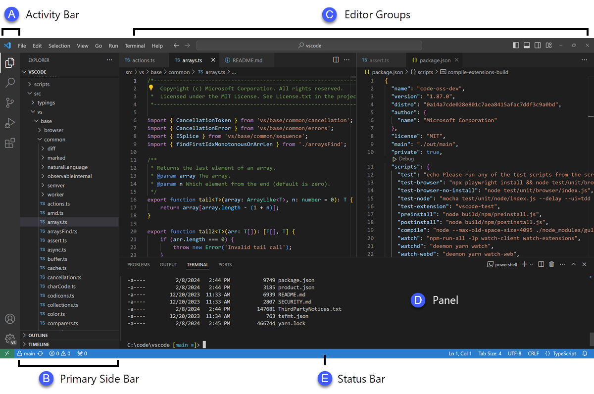
Figure 1:The VS Code interface: Explorer, editor, views, status bar, and integrated terminal. Image from the official VS Code user-interface tutorial.
For the first laboratory, use VS Code as an editor and as a convenient window on the terminal. The actual build commands are intentionally visible: this makes it easier to diagnose problems later on a remote machine or in a container.
3. The project layout
The relevant part of the repository is:
labs/lab-01/
├── CMakeLists.txt       # the build description for this small project
├── lab-01.cc            # the C++ source file
└── README.md            # a short description of the exercise
In the course repository the executable is built by the top-level
CMakeLists.txt. The standalone CMakeLists.txt shown below is the minimal
version of the same idea and can also be used in a separate personal copy.
cmake_minimum_required(VERSION 3.16)

project(lab01 LANGUAGES CXX)

set(CMAKE_CXX_STANDARD 17)
set(CMAKE_CXX_STANDARD_REQUIRED ON)
set(CMAKE_CXX_EXTENSIONS OFF)

add_executable(lab01 lab-01.cc)
The important distinction is between the source directory and the build directory. We do not put generated object files next to the source file.
4. A first C++ class template: Point<dim, Number>
Open labs/lab-01/lab-01.cc. The central example is the following class:
template <int dim, typename Number = double>
class Point
{
public:
  Number &operator[](std::size_t index)
  {
    return coordinates_.at(index);
  }

  const Number &operator[](std::size_t index) const
  {
    return coordinates_.at(index);
  }

private:
  std::array<Number, dim> coordinates_{};
};
There are two template parameters:
dimis a non-type template parameter. It fixes the number of coordinates at compile time;Numberis a type template parameter. It specifies the coordinate type and defaults todouble.
The following declarations therefore describe different types:
Point<2>        point_2d;
Point<3>        point_3d;
Point<2, float> point_2d_single_precision;
This pattern is already close to the style used by deal.II, where the spatial dimension is frequently a template parameter. At this stage we only need a small class with indexed access; constructors, iterators, and operator overloading can be introduced later.
The program also defines a templated function:
template <int dim, typename Number>
Number scalar_field(const Point<dim, Number> &point)
{
  static_assert(dim == 2, "This first example is two-dimensional.");
  constexpr Number pi = static_cast<Number>(3.14159265358979323846);
  return std::sin(pi * point[0]) * std::sin(pi * point[1]);
}
The function evaluates a scalar field on the unit square. The static_assert
is checked by the compiler and documents the limitation of this first example.
5. Configure, build, and run
The complete course repository contains other laboratories that depend on deal.II. To build only this introductory program without deal.II, use a separate build directory and disable the later laboratories:
cmake -S . -B build-lab01 -DNMPDE_BUILD_LABS=ON -DNMPDE_BUILD_DEALII_LABS=OFF -DNMPDE_BUILD_TESTS=OFF
cmake --build build-lab01 --target lab-01
Run the program from the repository root:
./build-lab01/bin/lab-01 output/field.csvThe program creates the output/ directory if necessary and writes a CSV file
with three columns:
x,y,u
0,0,0
0.05,0,0
...
The first two columns contain the point coordinates. The third column contains the value of the scalar field. Since CSV is plain text, open the generated file in VS Code and inspect it before moving to ParaView.
A useful diagnostic exercise
Change points_per_axis in the source file, rebuild, and run the program
again. Then deliberately introduce a small syntax error and observe how the
compiler reports the file and line number in the VS Code Problems view. Undo
the error and rebuild before continuing.
6. Reading the CSV file in ParaView
ParaView can open delimited text files. For an ordinary CSV file, the first
object is a table: each row is a sample and each named column is an array. To
give the rows spatial coordinates, use the Table to Points filter.
Open
output/field.csvwith File → Open.Press Apply in the Properties panel.
Select Filters → Table to Points.
Set
xas the X Column andyas the Y Column.Set the Z Column to
0or leave the points in the XY plane.Press Apply again.
Color the points using the
uarray.
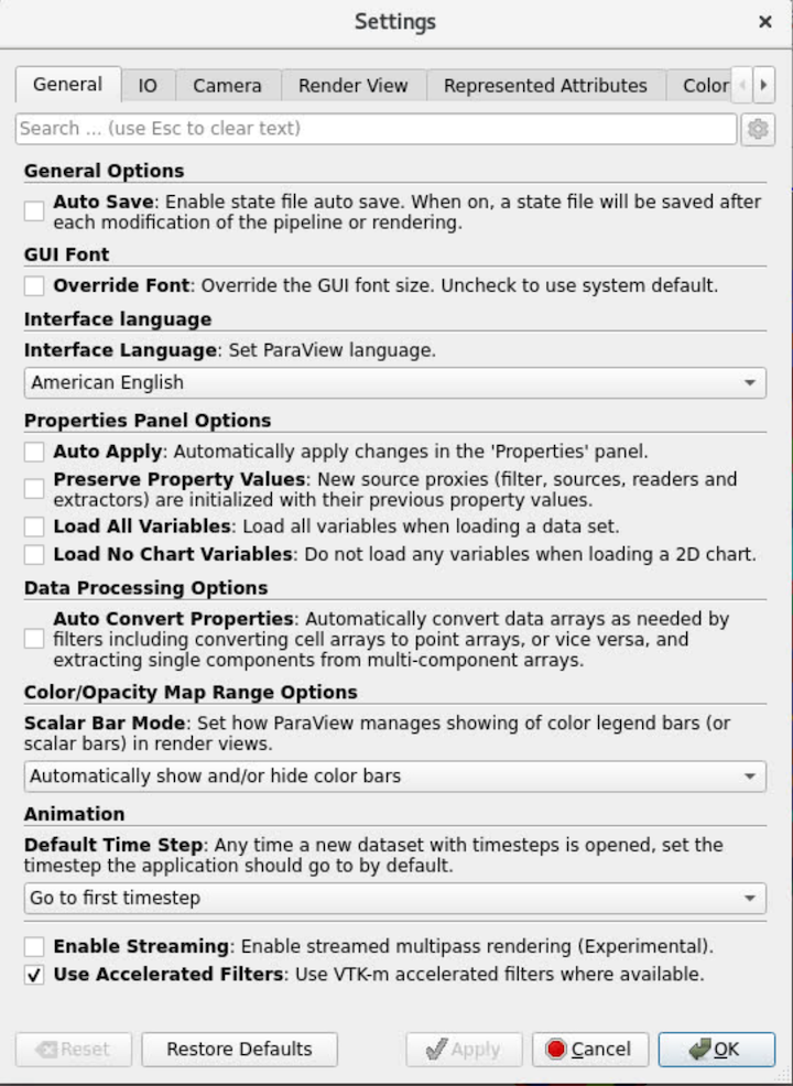
Figure 2:The basic ParaView pipeline and render view. Image from the official ParaView beginning GUI tutorial.
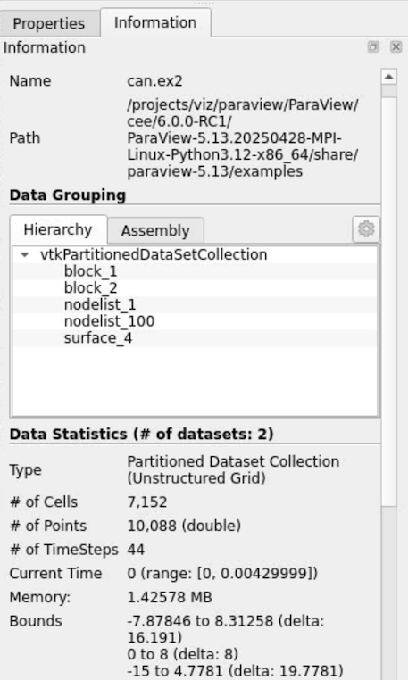
Figure 3:The Information tab is useful for checking the size and range of a data set. Image from the official ParaView beginning GUI tutorial.
The CSV format is intentionally simple, but it does not normally describe the
connectivity of a mesh. The result of Table to Points is therefore a point
cloud, not yet a finite element mesh or a continuous surface. This distinction
will become important when later laboratories write .vtu files from deal.II.
ParaView also provides Table to Structured Grid when a table contains enough
information to reconstruct a structured grid.
The official ParaView documentation provides further information about loading data and understanding tables and data sets.
From the CSV to contour lines
The point cloud can be converted into a triangular surface and then into
contour lines. Starting from the field.csv reader, build the following
pipeline:
CSV reader → Table to Points → Delaunay 2D → ContourSelect the
TableToPointsobject in the Pipeline Browser.Choose Filters → Alphabetical → Delaunay 2D and press Apply. The filter connects the points with triangles, producing a surface on which the scalar field can be interpolated.
Select
Delaunay2D1, choose Filters → Common → Contour, and press Apply.In the Contour properties, set Contour By to
u. Add one or more contour values, for example0.1,0.3,0.5, and0.7.Keep the Delaunay surface visible and color it by
u. SelectContour1, choose a contrasting solid color such as white, and increase Line Width if necessary.Toggle the visibility icons in the Pipeline Browser to compare the point cloud, triangulated surface, and contour lines.
The Contour filter extracts the points, curves, or surfaces where a scalar
field has a prescribed value. In this 2D case the output is a collection of
curves, one curve for each selected level. The filters therefore make the
geometry/data distinction explicit: Table to Points assigns coordinates,
Delaunay 2D creates connectivity, and Contour extracts level sets. See
the official ParaView filter tutorial
for the general contour workflow.
7. Previewing the course book locally
The repository contains the MyST source for the course book. Build the HTML pages from the repository root:
make siteThe generated pages are placed in notes/_build/html/. The Makefile
provides a serve target that starts Python’s standard HTTP server in that
directory:
make serveThe serve target depends on site, so it rebuilds the book first and then
starts the HTTP server.
Open http://127.0.0.1:8000/ in a browser. Keep the terminal running while
you inspect the page; press Ctrl+C to stop the server. If you change a MyST
file, rebuild the site with make site and refresh the browser.
8. Exercises
Exercise 1 — Change the field
Replace the scalar field with one of the following expressions and visualize the result:
u(x,y) = x + y
u(x,y) = x(1-x)y(1-y)
u(x,y) = cos(2 pi x) sin(pi y)
Explain which changes are made in the C++ source and which changes are visible only in the CSV output.
Exercise 2 — Change the scalar type
Instantiate the point as Point<2, float> and adapt the call to
scalar_field. Compare the generated values with the double version. Which
parts of the code depend on the Number template parameter?
Exercise 3 — Add a third coordinate
Create a Point<3> and initialize its three coordinates. Add a member function
that computes the squared Euclidean norm. Do not change the two-dimensional CSV
experiment yet; the goal is to practice the compile-time dimension parameter.
Exercise 4 — Use Git as a local safety net
If you are working in a personal copy, make a local commit after each milestone:
git status
git diff
git add labs/lab-01/lab-01.cc
git commit -m "Generate a scalar field in CSV format"
These commits are local checkpoints. They are not pushed to the lecturer’s repository.
Exercise 5 — Extend the program to three dimensions
Extend lab-01.cc so that it generates a three-dimensional data set.
Change the dimension to
dim = 3.Replace the two-dimensional restriction in
scalar_fieldwith a dimension- independent implementation, for example:Number value = 1; for (int d = 0; d < dim; ++d) value *= std::sin(pi * point[d]); return value;Add a loop over the third coordinate and assign
point[2].Change the CSV header to
x,y,z,uand write four values per row.Use a smaller grid such as
11points per axis for the first experiment: a three-dimensional grid contains11^3 = 1331points.
Write the result to a different file so that the original 2D experiment is preserved:
./build-lab01/bin/lab-01 output/field-3d.csvOpen the new file in ParaView and use Table to Points with x, y, and z
as the three coordinate columns. The 3D analogue of the previous pipeline is:
CSV reader → Table to Points → Delaunay 3D → ContourSelect Delaunay 3D instead of Delaunay 2D. Then apply Contour, choose
u, and experiment with several isovalues between zero and one. In three
dimensions the contour output is an isosurface rather than a curve.
Exercise 6 — Explore 3D opacity
Use the Display properties of the Delaunay surface and of the Contour output
to compare opacity values such as 1.0, 0.5, and 0.2. Try the following
experiments:
keep the triangulated volume almost transparent and the isosurfaces opaque;
keep the volume opaque and make the isosurfaces semi-transparent;
create several contour levels and use different colors or a different opacity for each level;
enable the opacity transfer function in the Color Map Editor, if available, and inspect how the visual result changes with the scalar value.
Record which objects are visible at each stage and explain why changing the opacity of the surface can reveal internal isosurfaces. ParaView’s contour filter is described as extracting an isosurface for a selected scalar value in the official basic-usage tutorial.
Completion checklist
Before leaving the laboratory, check that:
git pull --ff-onlycompleted successfully;the program builds from a clean
build-lab01directory;output/field.csvcontains the headerx,y,u;ParaView displays the samples after
Table to Points;the source contains both a
Point<dim, Number>class template and a templated scalar-field function;make sitecreatesnotes/_build/html/;make serveserves the local book.
The next laboratory will introduce a more structured C++ project and debugging before the first program that depends on deal.II.
A reference 2D contour plot
The following image was produced from the original field.csv with the
pipeline described above: Table to Points, Delaunay 2D, and Contour.
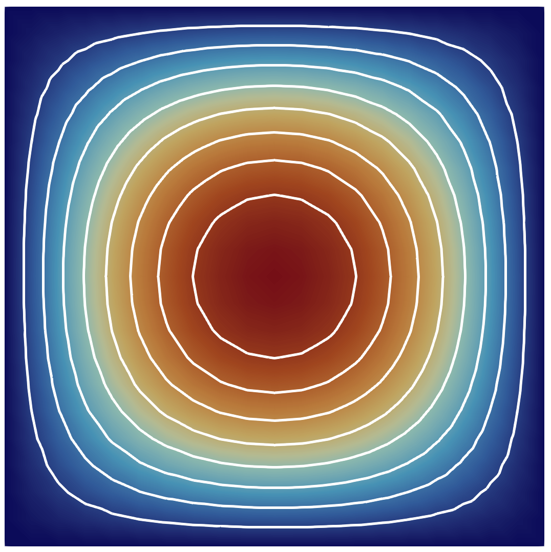
Figure 4:Reference contour plot for the 2D CSV data set. The filled colors show the scalar field, while the white curves are the selected contour levels.