ReducedPoisson
This tutorial explains the ReducedPoisson application from four angles:
the mathematical problem it solves;
how that problem is represented in the code;
how to run
app_reduced_poisson;how to write parameter files, from a single cylinder to a network.
The main implementation lives in include/reduced_poisson.h,
source/reduced_poisson.cc, include/reduced_coupling.h, and
source/tensor_product_space.cc.
What Problem Is Solved?
ReducedPoisson solves a Poisson problem in a bulk domain \(\Omega\), coupled to
an immersed lower-dimensional geometry \(\gamma\) through a reduced
Lagrange-multiplier formulation.
The bulk unknown is a scalar field
and the reduced geometry is typically a centerline stored in a VTK file, for
example data/tests/one_cylinder.vtk or data/medium_tree_8_3d.vtk.
The reduced geometry is not the actual coupling surface. Instead, the code:
reads a one-dimensional grid \(\gamma\);
picks a reference cross section \(D\);
selects a small set of cross-section basis functions \(\phi_i\);
sweeps that cross section along \(\gamma\);
uses the tensor-product space on \(\gamma \times D\) as the multiplier space.
This gives an immersed two-dimensional interface in 3D, or an immersed one-dimensional interface in 2D, without meshing that interface explicitly in the background grid.
Continuous Formulation
Let \(f\) be the bulk forcing, let \(u_D\) be the Dirichlet data on the selected outer boundary ids, and let
be the reduced target value on the immersed interface generated from \(\gamma\) and \(D\).
The problem solved by ReducedPoisson is:
The constraint on \(\Gamma_\gamma\) is enforced with a reduced multiplier \(\lambda \in Q_{\mathrm{red}}\). The weak form is:
and
Here \(X(s,y)\) maps reduced coordinates on \(\gamma \times D\) to physical points on the immersed interface.
The crucial approximation is that both the multiplier and the interface data are represented with only a few transverse modes:
That is the reduction.
Discrete Block System
After discretization, the code solves
In the implementation:
Ais the bulk Poisson stiffness matrix assembled insource/reduced_poisson.cc.Bis the reduced trace/projection operator assembled ininclude/reduced_coupling.h.gis the reduced right-hand side assembled ininclude/reduced_coupling.h.the Schur or augmented-Lagrangian solve is implemented in
source/reduced_poisson.cc.
So the program is not computing a forcing generated by the network. It is computing a bulk harmonic or forced scalar field whose trace matches prescribed reduced data on the immersed interface.
How The Geometry Is Built
The reduced geometry comes from a VTK file representing a one-dimensional mesh.
For each quadrature point on that mesh, the code creates physical quadrature
points on the immersed interface by transforming the reference cross section.
This happens in source/tensor_product_space.cc.
In practice:
in 3D, the reduced grid is a centerline and the interface is a tube surface;
in 2D, the reduced grid is a curve and the interface is a pair of offset points generated from the one-dimensional reference cross section.
The local interface thickness can be:
constant, via
Representative domain/Thickness;read from the reduced VTK file through a point field, via
Representative domain/Thickness field name.
For example, data/tests/one_cylinder_properties.vtk contains a field named
radius.
How To Run The Program
The entry point is apps/app_reduced_poisson.cc.
After building the project, run:
./build/reduced_poisson[_debug] ../tutorials/reduced_poisson/<input_file.prm>
The program decides whether to instantiate the 2D or 3D version from the parameter-file name itself:
if the filename contains the substring
3d, it runsReducedPoisson<3>;otherwise it runs
ReducedPoisson<2>.
This behavior comes directly from apps/app_reduced_poisson.cc. In practice,
name 3D input files something like my_case_3d.prm.
Typical Output
Each run writes:
a bulk solution file for each cycle such as
solution_0.vtu;a particle/interface file for each cycle such as
solution_particles_0.vtu;a
.pvdcollection for both outputs;a dumped parameter file
used_parameters_*.prm.
This is handled in source/reduced_poisson.cc.
Anatomy Of The Parameter File
The main section is:
subsection Reduced Poisson
  ...
end
Inside it, the most important groups are:
Bulk problem
These parameters define the background PDE and mesh:
FE degree: polynomial degree of the bulk FE space.Dirichlet boundary ids: boundary ids where \(u = u_D\) is imposed.Grid generation/Grid generator: bulk mesh type or input file.Grid generation/Grid generator arguments: arguments for the grid generator.Right hand side: the bulk forcing \(f\).Dirichlet boundary conditions: the outer boundary value \(u_D\).
Bulk refinement and output
Output directoryOutput nameOutput results also before solvingRefinement and remeshing/*
These affect postprocessing and adaptive refinement of the bulk mesh only.
Linear solver
Solver type: currentlySchurorAL.Assemble full AL system: whether to build the augmented operator explicitly in the augmented-Lagrangian path.Solver/Inner controlSolver/Outer control
Schur follows the explicit Schur-complement path. AL uses the
augmented-Lagrangian preconditioned solve.
Reduced coupling
The reduced interface data comes from the Reduced coupling subtree:
Representative domain/Reduced grid name: the VTK file containing the reduced geometry.Representative domain/Finite element degree: FE degree along the reduced manifold \(\gamma\).Representative domain/Quadrature type: 1D quadrature family used byQuadratureSelectorbefore applying the iterated rule. The default isgauss.Representative domain/Number of quadrature points: quadrature order on \(\gamma\).Representative domain/Number of quadrature repetitions: how many times to repeat the reduced-cell Gauss quadrature. The default value1keeps the standard Gauss rule.Representative domain/Thickness: constant radius or half-thickness.Representative domain/Thickness field name: field to read from the VTK file instead of a constant thickness.Representative domain/Reduced right hand side: the coefficient functions \(\bar g_i(s)\) for the reduced target data.
Cross-section basis
These live in the nested Cross section subsection:
Maximum inclusion degree: polynomial degree used to generate transverse basis functions.Selected indices: which transverse modes are kept.Inclusion type: currentlyhyper_ballorhyper_cube.Refinement level: resolution of the reference cross section.
If you keep only Selected indices = 0, the interface data are reduced to one
transverse mode. If you keep more indices, the interface data can vary in the
cross section with higher fidelity.
Reduced-grid preprocessing
These are the Local refinement parameters:
Refinement strategySpace pre-refinement cyclesEmbedded pre-refinement cyclesSpace post-refinement cyclesEmbedded post-refinement cyclesRefinement factorMax refinement level
They control how the reduced grid and the background grid are balanced before coupling.
Particle lookup
Under Particle coupling:
RTree extraction level
This controls how aggressively the bounding-box search structure is compressed before particles are inserted into the background mesh.
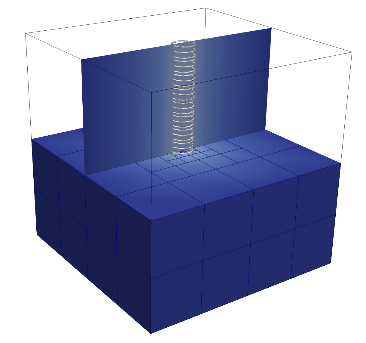
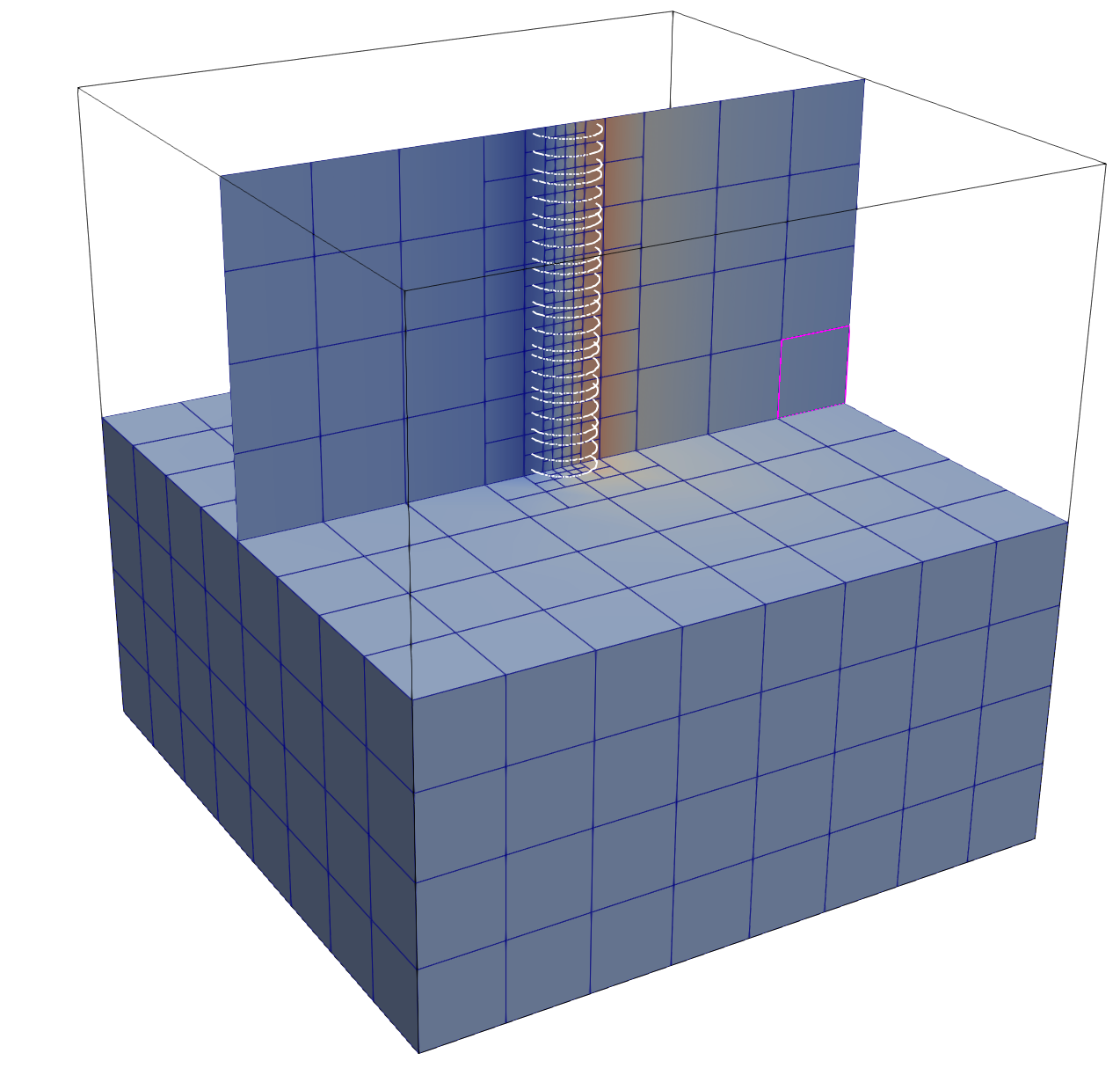
A Minimal 3D Single-Cylinder Example
This is the simplest useful ReducedPoisson<3> setup:
cube background domain
[-1,1]^3;zero outer Dirichlet boundary;
one straight cylinder centerline;
one reduced transverse mode;
constant target value \(g = 1\) on the immersed interface.
The actual tutorial input file is stored at
tutorials/reduced_poisson/single_cylinder_3d.prm:
subsection Reduced Poisson
  set Assemble full AL system            = false
  set Dirichlet boundary ids             = 0,1,2,3,4
  set FE degree                          = 1
  set Output directory                   = ./output/reduced_poisson_single_cylinder
  set Output name                        = single_cylinder
  set Output results also before solving = false
  set Solver type                        = AL
  subsection Dirichlet boundary conditions
    set Function constants  =
    set Function expression = 0
    set Variable names      = x,y,z,t
  end
  subsection Grid generation
    set Grid generator           = hyper_cube
    set Grid generator arguments = 0: 1: true
  end
  subsection Refinement and remeshing
    set Coarsening fraction         = 0.0
    set Maximum number of cells     = 20000
    set Number of refinement cycles = 1
    set Refinement fraction         = 0.3
    set Strategy                    = fixed_fraction
  end
  subsection Right hand side
    set Function constants  =
    set Function expression = 0
    set Variable names      = x,y,z,t
  end
  subsection Solver
    subsection Inner control
      set Log frequency = 1
      set Log history   = false
      set Log result    = true
      set Max steps     = 200
      set Reduction     = 1e-10
      set Tolerance     = 1e-12
    end
    subsection Outer control
      set Log frequency = 1
      set Log history   = false
      set Log result    = true
      set Max steps     = 200
      set Reduction     = 1e-10
      set Tolerance     = 1e-12
    end
  end
end
subsection Reduced coupling
  subsection Cross section
    set Inclusion type           = hyper_ball
    set Maximum inclusion degree = 0
    set Refinement level         = 4
    set Selected indices         = 0
  end
  subsection Local refinement parameters
    set Embedded post-refinement cycles = 0
    set Embedded pre-refinement cycles  = 4
    set Max refinement level            = 10
    set Refinement factor               = 1
    set Refinement strategy             = space
    set Space post-refinement cycles    = 3
    set Space pre-refinement cycles     = 1
  end
  subsection Particle coupling
    set RTree extraction level = 1
  end
  subsection Representative domain
    set Finite element degree       = 1
    set Quadrature type             = trapez
    set Number of quadrature repetitions = 3
    set Reduced grid name           = ../data/tests/one_cylinder.vtk
    set Reduced right hand side     = 1
    set Thickness                   = 0.05
    set Thickness field name        =
  end
end
subsection Error
  set Enable computation of the errors = true
  set Error file name                  =
  set Error precision                  = 3
  set Exponent for p-norms             = 2
  set Extra columns                    = cells, dofs
  set List of error norms to compute   = L2_norm, Linfty_norm, H1_norm
  set Rate key                         = dofs
  set Rate mode                        = reduction_rate_log2
end
Run it with:
./build/reduced_poisson single_cylinder_3d.prm
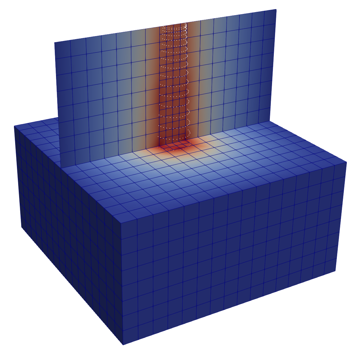
What this computes:
the bulk equation is \(-\Delta u = 0\);
the outer cube boundary is fixed at zero on all lateral faces, and the top and bottom faces are treated as homogeneous Neumann boundaries;
along the swept cylinder interface, the average reduced trace is driven toward
1;with only one transverse basis function, the interface condition is the simplest possible reduced one.
Single Cylinder With Variable Radius
The next step is to read radius data from the VTK file instead of using a constant thickness.
The file data/tests/one_cylinder_properties.vtk contains a field named
radius. The corresponding tutorial input file is
tutorials/reduced_poisson/single_cylinder_variable_radius_3d.prm:
subsection Reduced Poisson
  set Assemble full AL system            = false
  set Dirichlet boundary ids             = 0,1,2,3,4
  set FE degree                          = 1
  set Output directory                   = ./output/reduced_poisson_single_cylinder_variable_radius
  set Output name                        = single_cylinder_variable_radius
  set Output results also before solving = false
  set Solver type                        = AL
  subsection Dirichlet boundary conditions
    set Function constants  =
    set Function expression = 0
    set Variable names      = x,y,z,t
  end
  subsection Grid generation
    set Grid generator           = hyper_cube
    set Grid generator arguments = 0: 1: true
  end
  subsection Refinement and remeshing
    set Coarsening fraction         = 0.0
    set Maximum number of cells     = 20000
    set Number of refinement cycles = 1
    set Refinement fraction         = 0.3
    set Strategy                    = fixed_fraction
  end
  subsection Right hand side
    set Function constants  =
    set Function expression = 0
    set Variable names      = x,y,z,t
  end
  subsection Solver
    subsection Inner control
      set Log frequency = 1
      set Log history   = false
      set Log result    = true
      set Max steps     = 200
      set Reduction     = 1e-10
      set Tolerance     = 1e-12
    end
    subsection Outer control
      set Log frequency = 1
      set Log history   = false
      set Log result    = true
      set Max steps     = 200
      set Reduction     = 1e-10
      set Tolerance     = 1e-12
    end
  end
end
subsection Reduced coupling
  subsection Cross section
    set Inclusion type           = hyper_ball
    set Maximum inclusion degree = 0
    set Refinement level         = 3
    set Selected indices         = 0
  end
  subsection Local refinement parameters
    set Embedded post-refinement cycles = 0
    set Embedded pre-refinement cycles  = 0
    set Max refinement level            = 10
    set Refinement factor               = 1
    set Refinement strategy             = space
    set Space post-refinement cycles    = 1
    set Space pre-refinement cycles     = 4
  end
  subsection Particle coupling
    set RTree extraction level = 1
  end
  subsection Representative domain
    set Finite element degree       = 1
    set Quadrature type             = trapez
    set Number of quadrature repetitions = 33
    set Reduced grid name           = ../data/tests/one_cylinder_properties.vtk
    set Reduced right hand side     = 1
    set Thickness                   = 0.05
    set Thickness field name        = radius
  end
end
subsection Error
  set Enable computation of the errors = true
  set Error file name                  =
  set Error precision                  = 3
  set Exponent for p-norms             = 2
  set Extra columns                    = cells, dofs
  set List of error norms to compute   = L2_norm, Linfty_norm, H1_norm
  set Rate key                         = dofs
  set Rate mode                        = reduction_rate_log2
end
Here:
Thicknessacts as a fallback value;Thickness field name = radiustells the code to read the point field namedradius;the local cross-section measure in both the reduced mass matrix and reduced right-hand side is scaled accordingly.
Single Cylinder With More Transverse Modes
To allow nontrivial variation across the cross section, increase the polynomial
degree and keep more selected modes. The corresponding tutorial input file is
tutorials/reduced_poisson/single_cylinder_multimode_3d.prm:
subsection Reduced Poisson
  set Assemble full AL system            = false
  set Dirichlet boundary ids             = 0,1,2,3,4
  set FE degree                          = 1
  set Output directory                   = ./output/reduced_poisson_single_cylinder_multimode
  set Output name                        = single_cylinder_multimode
  set Output results also before solving = false
  set Solver type                        = Schur
  subsection Dirichlet boundary conditions
    set Function constants  =
    set Function expression = 0
    set Variable names      = x,y,z,t
  end
  subsection Grid generation
    set Grid generator           = hyper_cube
    set Grid generator arguments = 0: 1: true
  end
  subsection Refinement and remeshing
    set Coarsening fraction         = 0.0
    set Maximum number of cells     = 20000
    set Number of refinement cycles = 1
    set Refinement fraction         = 0.3
    set Strategy                    = fixed_fraction
  end
  subsection Right hand side
    set Function constants  =
    set Function expression = 0
    set Variable names      = x,y,z,t
  end
  subsection Solver
    subsection Inner control
      set Log frequency = 1
      set Log history   = false
      set Log result    = true
      set Max steps     = 200
      set Reduction     = 1e-10
      set Tolerance     = 1e-12
    end
    subsection Outer control
      set Log frequency = 1
      set Log history   = false
      set Log result    = true
      set Max steps     = 200
      set Reduction     = 1e-10
      set Tolerance     = 1e-12
    end
  end
end
subsection Reduced coupling
  subsection Cross section
    set Inclusion type           = hyper_ball
    set Maximum inclusion degree = 1
    set Refinement level         = 3
    set Selected indices         = 0, 1, 2
  end
  subsection Local refinement parameters
    set Embedded post-refinement cycles = 0
    set Embedded pre-refinement cycles  = 4
    set Max refinement level            = 10
    set Refinement factor               = 1
    set Refinement strategy             = space
    set Space post-refinement cycles    = 1
    set Space pre-refinement cycles     = 3
  end
  subsection Particle coupling
    set RTree extraction level = 1
  end
  subsection Representative domain
    set Finite element degree       = 1
    set Quadrature type             = trapez
    set Number of quadrature repetitions = 3
    set Reduced grid name           = ../data/tests/one_cylinder.vtk
    set Reduced right hand side     = 1; 1; 2
    set Thickness                   = 0.05
    set Thickness field name        =
  end
end
subsection Error
  set Enable computation of the errors = true
  set Error file name                  =
  set Error precision                  = 3
  set Exponent for p-norms             = 2
  set Extra columns                    = cells, dofs
  set List of error norms to compute   = L2_norm, Linfty_norm, H1_norm
  set Rate key                         = dofs
  set Rate mode                        = reduction_rate_log2
end
Interpretation:
mode
0is usually the constant transverse mode;the additional entries activate higher-order cross-sectional content;
the length of
Reduced right hand sidemust match the number of selected basis functions for the scalar problem.
This is the first setting where the reduced interface condition is more than a simple averaged trace.
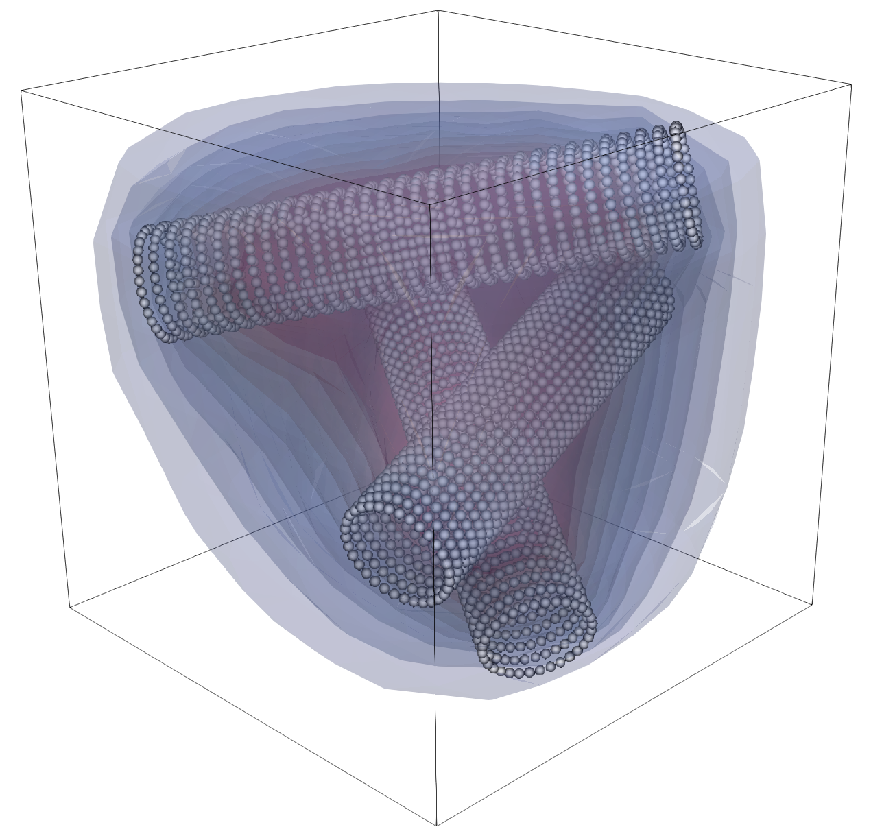
Three-Cylinder Example
A slightly richer geometry is provided by the three-cylinder reduced grids such
as data/three_cylinders_R005.vtk.
A representative parameter file is stored at
tutorials/reduced_poisson/three_cylinders_3d.prm:
subsection Reduced Poisson
  set Assemble full AL system            = false
  set Dirichlet boundary ids             = 0
  set FE degree                          = 1
  set Output directory                   = ./output/reduced_poisson_three_cylinders
  set Output name                        = three_cylinders
  set Output results also before solving = false
  set Solver type                        = AL
  subsection Dirichlet boundary conditions
    set Function constants  =
    set Function expression = 0
    set Variable names      = x,y,z,t
  end
  subsection Grid generation
    set Grid generator           = hyper_cube
    set Grid generator arguments = -1: 1: false
  end
  subsection Refinement and remeshing
    set Coarsening fraction         = 0
    set Maximum number of cells     = 20000
    set Number of refinement cycles = 1
    set Refinement fraction         = 0.3
    set Strategy                    = fixed_fraction
  end
  subsection Right hand side
    set Function constants  =
    set Function expression = 0
    set Variable names      = x,y,z,t
  end
  subsection Solver
    subsection Inner control
      set Log frequency = 1
      set Log history   = false
      set Log result    = true
      set Max steps     = 100
      set Reduction     = 1.e-10
      set Tolerance     = 1.e-10
    end
    subsection Outer control
      set Log frequency = 1
      set Log history   = false
      set Log result    = true
      set Max steps     = 100
      set Reduction     = 1.e-2
      set Tolerance     = 1.e-10
    end
  end
end
subsection Reduced coupling
  subsection Cross section
    set Inclusion type           = hyper_ball
    set Maximum inclusion degree = 0
    set Refinement level         = 3
    set Selected indices         =
  end
  subsection Local refinement parameters
    set Embedded post-refinement cycles = 0
    set Embedded pre-refinement cycles  = 0
    set Max refinement level            = 10
    set Refinement factor               = 1
    set Refinement strategy             = space
    set Space post-refinement cycles    = 1
    set Space pre-refinement cycles     = 3
  end
  subsection Particle coupling
    set RTree extraction level = 1
  end
  subsection Representative domain
    set Finite element degree            = 1
    set Number of quadrature points      = 0
    set Number of quadrature repetitions = 32
    set Quadrature type                  = trapez
    set Reduced grid name                = ../data/three_cylinders_R005.vtk
    set Reduced right hand side          = 1
    set Thickness                        = 0.2
    set Thickness field name             =
  end
end
subsection Error
  set Enable computation of the errors = true
  set Error file name                  =
  set Error precision                  = 3
  set Exponent for p-norms             = 2
  set Extra columns                    = cells, dofs
  set List of error norms to compute   = L2_norm, Linfty_norm, H1_norm
  set Rate key                         = dofs
  set Rate mode                        = reduction_rate_log2
end
Compared with the single-cylinder case, only the reduced geometry changes. That is one of the main advantages of this workflow: the bulk solver and background mesh setup stay the same while the embedded geometry can become much more complex.
Complex Network Example
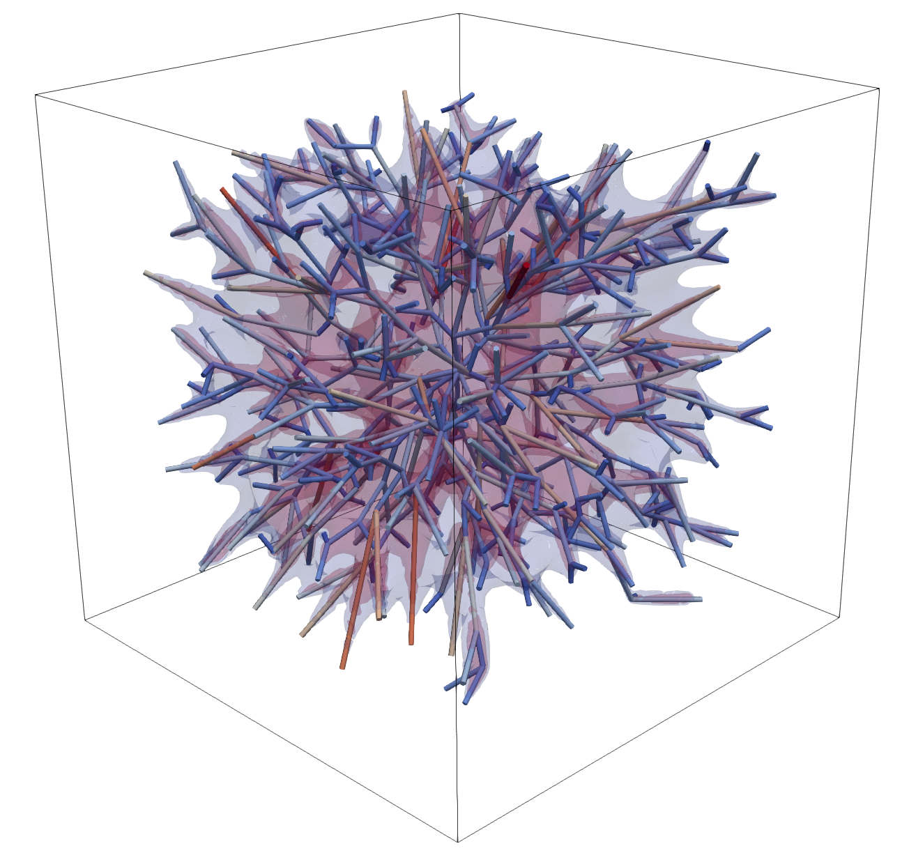
For a network-scale case, use a real tree-like reduced grid such as
data/medium_tree_8_3d.vtk.
A practical starting point is stored at
tutorials/reduced_poisson/medium_tree_3d.prm:
subsection Reduced Poisson
  set Assemble full AL system            = false
  set Dirichlet boundary ids             = 0
  set FE degree                          = 1
  set Output directory                   = ./output/reduced_poisson_medium_tree
  set Output name                        = medium_tree
  set Output results also before solving = false
  set Solver type                        = AL
  subsection Dirichlet boundary conditions
    set Function constants  =
    set Function expression = 0
    set Variable names      = x,y,z,t
  end
  subsection Grid generation
    set Grid generator           = hyper_cube
    set Grid generator arguments = -1: 1: false
  end
  subsection Refinement and remeshing
    set Coarsening fraction         = 0.0
    set Maximum number of cells     = 50000
    set Number of refinement cycles = 1
    set Refinement fraction         = 0.15
    set Strategy                    = fixed_fraction
  end
  subsection Right hand side
    set Function constants  =
    set Function expression = 0
    set Variable names      = x,y,z,t
  end
  subsection Solver
    subsection Inner control
      set Log frequency = 1
      set Log history   = false
      set Log result    = true
      set Max steps     = 300
      set Reduction     = 1e-2
      set Tolerance     = 1e-12
    end
    subsection Outer control
      set Log frequency = 1
      set Log history   = false
      set Log result    = true
      set Max steps     = 200
      set Reduction     = 1e-8
      set Tolerance     = 1e-10
    end
  end
end
subsection Reduced coupling
  subsection Cross section
    set Inclusion type           = hyper_ball
    set Maximum inclusion degree = 0
    set Refinement level         = 1
    set Selected indices         = 0
  end
  subsection Local refinement parameters
    set Embedded post-refinement cycles = 0
    set Embedded pre-refinement cycles  = 0
    set Max refinement level            = 10
    set Refinement factor               = 1
    set Refinement strategy             = space
    set Space post-refinement cycles    = 2
    set Space pre-refinement cycles     = 4
  end
  subsection Particle coupling
    set RTree extraction level = 1
  end
  subsection Representative domain
    set Finite element degree            = 1
    set Number of quadrature points      = 3
    set Number of quadrature repetitions = 32
    set Quadrature type                  = trapez
    set Reduced grid name                = ../data/medium_tree_8_3d.vtk
    set Reduced right hand side          = 1
    set Thickness                        = 0.01
    set Thickness field name             =
  end
end
subsection Error
  set Enable computation of the errors = true
  set Error file name                  =
  set Error precision                  = 3
  set Exponent for p-norms             = 2
  set Extra columns                    = cells, dofs
  set List of error norms to compute   = L2_norm, Linfty_norm, H1_norm
  set Rate key                         = dofs
  set Rate mode                        = reduction_rate_log2
end
For this class of example:
use
ALbeforeSchurunless you have a specific reason not to;start with one transverse mode;
keep the reduced FE degree low initially;
use adaptive bulk refinement only after the geometry and solver settings are stable.
How To Read A ReducedPoisson Parameter File
A good reading order is:
Reduced Poisson: define the bulk PDE and the solver.Reduced coupling/Representative domain/Reduced right hand side: define what trace you want on the immersed interface.Representative domain: define where the reduced geometry lives and how it is discretized.Cross section: define how rich the transverse basis is.Local refinement parametersandParticle coupling: tune geometric robustness and search behavior.
This order mirrors the code:
build the bulk mesh;
build the reduced space;
create immersed quadrature particles;
assemble
A,B, andg;solve the block system.
Common Pitfalls
If a 3D run starts the 2D executable path, check the filename. It must contain
3d.If
Reduced right hand sidehas the wrong number of entries, checkCross section/Selected indices.If the reduced geometry seems too thick or too thin, check whether thickness comes from
Thicknessor fromThickness field name.If the coupling looks weak or noisy, increase the reduced quadrature points before increasing the bulk FE degree.
If the network case becomes expensive, first reduce the number of transverse modes, then reduce bulk refinement, and only then change solver settings.