This lecture introduces the variational point of view that will be used throughout the course. We start from a model elliptic problem, derive its weak formulation, and then restrict the problem to a finite-dimensional space. The main results are the Lax–Milgram lemma, Galerkin orthogonality, and Céa’s lemma.
1. A model problem
Let be a bounded domain with sufficiently regular boundary . We consider the Poisson problem with homogeneous Dirichlet boundary conditions:
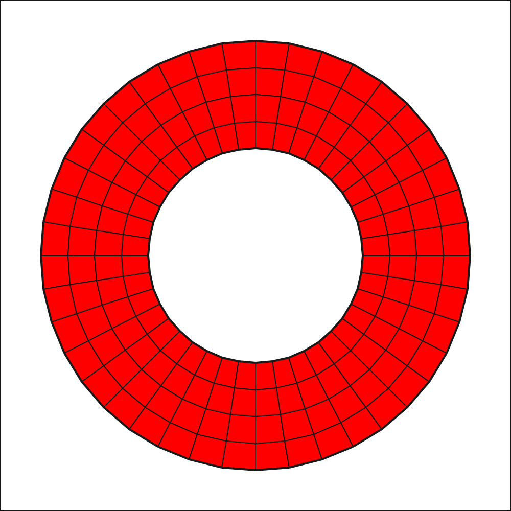
Figure 1:Mesh generated by the course test suite.
Here is the given source term and is the unknown solution. This is a useful model problem because it contains the main ingredients of elliptic finite element methods while remaining simple enough to analyze explicitly.
There are two broad ways to obtain a numerical approximation:
discretize the differential operator directly, as in finite-difference methods;
keep the differential operator in a weak form and approximate the space in which the solution is sought, as in finite-element methods.
The second point of view is particularly useful on non-rectangular domains and when the data or the solution are not smooth enough for the strong equation to be interpreted pointwise.
2. The weak formulation
Let be a smooth test function that vanishes on the boundary. Multiplying (1) by , integrating over , and integrating by parts gives
The boundary term vanishes because both and have zero trace. The natural space for this problem is
and the weak problem is:
where
The right-hand side is written as a duality pairing because, in general, the data may belong to , the dual of , rather than to .
3. Well-posedness and the Lax–Milgram lemma
The abstract form of the problem is determined by a bilinear form and a functional . Two properties are central:
boundedness: there is a constant such that for all ;
coercivity: there is a constant such that for all .
For the Poisson problem, boundedness follows from the Cauchy–Schwarz inequality:
On , Poincaré’s inequality makes the seminorm equivalent to the -norm. Hence the form is also coercive, and the weak Poisson problem has a unique solution.
4. The Ritz–Galerkin approximation
Let be a finite-dimensional conforming space. The Galerkin approximation is obtained by restricting the weak problem to :
Because the same boundedness and coercivity estimates hold on the subspace , the discrete problem is also uniquely solvable.
Choose a basis of and write
Testing (9) with each basis function gives the linear system
Thus the stiffness matrix and load vector are
When is symmetric, as for the Poisson problem, is symmetric positive definite. This is the algebraic form of the Ritz–Galerkin method.
The Ritz interpretation
For a symmetric bilinear form, define the energy functional
The solution of the continuous problem is the unique minimizer of over , while is the unique minimizer over :
The term Ritz emphasizes this minimization property; Galerkin emphasizes the orthogonality condition that characterizes the discrete solution.
5. Galerkin orthogonality
The exact solution also satisfies the weak equation for every , since . Subtracting the discrete equation gives
This is Galerkin orthogonality: the error is orthogonal to the discrete space with respect to the bilinear form . It is the key identity behind the basic a priori error estimate.
6. Céa’s lemma
The estimate separates the analysis into two parts:
measures the stability of the variational problem;
the infimum measures the best approximation available in .
To see the mechanism, take any . By coercivity and Galerkin orthogonality,
After cancelling the error norm and taking the infimum over , we obtain Céa’s estimate.
For finite elements, this result reduces the error analysis to an approximation question: how well can the exact solution be approximated by the chosen finite element space? The following lectures will address the construction of these spaces and the estimates needed to answer that question.
Summary
The weak formulation replaces the strong differential equation with an equation in a function space.
Lax–Milgram gives existence, uniqueness, and stability under boundedness and coercivity.
The Ritz–Galerkin method restricts the variational problem to a finite- dimensional conforming space.
Galerkin orthogonality is the fundamental error identity.
Céa’s lemma bounds the numerical error by the best approximation error in the discrete space.