This notebook tests the reduced formulation from the previous lecture on a deliberately nonsmooth target state: a rectangular step function. The target is not in , so it cannot be reproduced exactly by an elliptic state, but it is still a perfectly meaningful tracking target in .
from pathlib import Path
import sys

import matplotlib.pyplot as plt
from matplotlib.animation import PillowWriter, FuncAnimation
import numpy as np
from IPython.display import Image


def find_codes_dir() -> tuple[Path, Path]:
    cwd = Path.cwd().resolve()

    # First try: current directory and its parents.
    for base in [cwd, *cwd.parents]:
        candidate = base / "jupyterbook" / "codes"
        if (candidate / "common").exists():
            return candidate, candidate / "lecture04"
        candidate = base / "codes"
        if (candidate / "common").exists() and (candidate / "lecture04").exists():
            return candidate, candidate / "lecture04"

    # Second try: recursive search below the current working directory.
    for candidate in cwd.glob("**/jupyterbook/codes"):
        if (candidate / "common").exists() and (candidate / "lecture04").exists():
            return candidate.resolve(), (candidate / "lecture04").resolve()
    for candidate in cwd.glob("**/codes"):
        if (candidate / "common").exists() and (candidate / "lecture04").exists():
            return candidate.resolve(), (candidate / "lecture04").resolve()

    raise RuntimeError(
        "Could not locate the 'jupyterbook/codes' directory. "
        "Open the notebook inside the repository or set the working directory accordingly."
    )


CODES_DIR, NOTEBOOK_DIR = find_codes_dir()

if str(CODES_DIR) not in sys.path:
    sys.path.insert(0, str(CODES_DIR))

from common.elliptic_control_1d import ReducedPoissonControl1D, reduced_steepest_descent_history
from common.fd1d import UniformGrid1D
Problem setup
grid = UniformGrid1D(num_interior=200)
x = grid.x

target = np.where((x >= 0.35) & (x <= 0.65), 1.0, 0.0)
alpha = 1.0e-3

problem = ReducedPoissonControl1D(
    grid=grid,
    alpha=alpha,
    desired_state=target,
)

control0 = np.zeros_like(x)
history = reduced_steepest_descent_history(problem, control0, max_iter=60)

print(f"stored iterates: {len(history)}")
print(f"initial cost:    {history[0].value:.6e}")
print(f"final cost:      {history[-1].value:.6e}")
print(f"final grad norm: {history[-1].gradient_norm:.6e}")
stored iterates: 16
initial cost: 1.492537e-01
final cost: 6.875749e-02
final grad norm: 9.547540e-11
Initial and final configurations
def plot_snapshot(ax_state, ax_control, item, title):
    ax_state.plot(x, target, color="black", linestyle="--", linewidth=2.0, label="target $y_d$")
    ax_state.plot(x, item.state, color="tab:blue", linewidth=2.0, label="state $y$")
    ax_state.set_title(title)
    ax_state.set_ylabel("state")
    ax_state.set_xlim(0.0, 1.0)
    ax_state.set_ylim(-0.05, 1.15)
    ax_state.grid(True, alpha=0.25)
    ax_state.legend(loc="upper right")

    ax_control.plot(x, item.control, color="tab:red", linewidth=2.0, label="control $u$")
    ax_control.set_xlabel("$x$")
    ax_control.set_ylabel("control")
    ax_control.set_xlim(0.0, 1.0)
    ax_control.grid(True, alpha=0.25)
    ax_control.legend(loc="upper right")


fig, axes = plt.subplots(2, 2, figsize=(12, 6), sharex="col")
plot_snapshot(axes[0, 0], axes[1, 0], history[0], "Initial iterate")
plot_snapshot(axes[0, 1], axes[1, 1], history[-1], "Final iterate")
fig.suptitle("Tracking a rectangular $L^2$ target with an elliptic state", fontsize=14)
fig.tight_layout()
plt.show()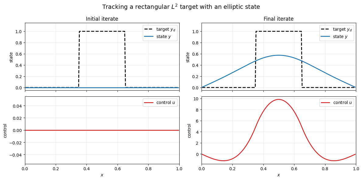
Cost decrease
fig, ax = plt.subplots(figsize=(7, 4))
ax.semilogy([item.value for item in history], marker="o", linewidth=1.5)
ax.set_xlabel("iteration")
ax.set_ylabel("$J(u^k)$")
ax.set_title("Reduced cost along steepest descent")
ax.grid(True, alpha=0.3)
plt.show()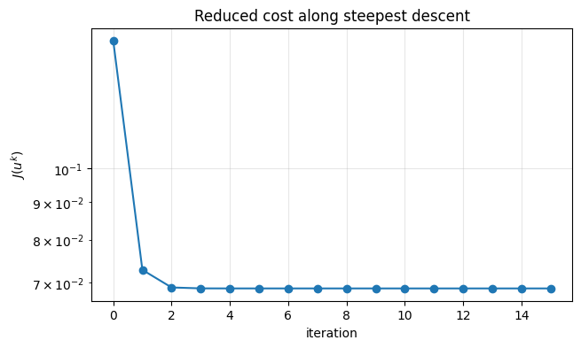
Animation of the state approaching the target
assets_dir = NOTEBOOK_DIR / "assets"
assets_dir.mkdir(parents=True, exist_ok=True)
gif_path = assets_dir / "lecture04_step_target.gif"

frame_stride = max(1, len(history) // 25)
frames = history[::frame_stride]
if frames[-1].iteration != history[-1].iteration:
    frames.append(history[-1])

fig, (ax_state, ax_control) = plt.subplots(2, 1, figsize=(8, 6), sharex=True)

ax_state.plot(x, target, "k--", linewidth=2.0, label="target $y_d$")
state_line, = ax_state.plot([], [], color="tab:blue", linewidth=2.5, label="state $y^k$")
ax_state.set_xlim(0.0, 1.0)
ax_state.set_ylim(-0.05, 1.15)
ax_state.set_ylabel("state")
ax_state.grid(True, alpha=0.25)
ax_state.legend(loc="upper right")

control_line, = ax_control.plot([], [], color="tab:red", linewidth=2.0, label="control $u^k$")
ax_control.set_xlim(0.0, 1.0)
u_min = min(np.min(item.control) for item in history)
u_max = max(np.max(item.control) for item in history)
pad = 0.05 * max(1.0, u_max - u_min)
ax_control.set_ylim(u_min - pad, u_max + pad)
ax_control.set_xlabel("$x$")
ax_control.set_ylabel("control")
ax_control.grid(True, alpha=0.25)
ax_control.legend(loc="upper right")

title = fig.suptitle("")

def init():
    state_line.set_data([], [])
    control_line.set_data([], [])
    title.set_text("")
    return state_line, control_line, title


def update(item):
    state_line.set_data(x, item.state)
    control_line.set_data(x, item.control)
    title.set_text(
        f"Iteration {item.iteration}: "
        f"J={item.value:.3e}, "
        f"||grad J||={item.gradient_norm:.3e}"
    )
    return state_line, control_line, title


animation = FuncAnimation(
    fig,
    update,
    frames=frames,
    init_func=init,
    interval=250,
    blit=True,
)
animation.save(gif_path, writer=PillowWriter(fps=4))
plt.close(fig)

print(f"saved animation to {gif_path}")
Image(filename=str(gif_path))
saved animation to /home/runner/work/nmopt/nmopt/jupyterbook/codes/lecture04/assets/lecture04_step_target.gif
Final remarks
The target is discontinuous, so it is not an function.
The state remains smooth because it solves an elliptic equation.
The optimizer compensates by creating a control concentrated near the jump locations.
This is exactly the kind of example where the reduced formulation is easy to test numerically.