Finite-dimensional conceptual experiments for:
Gradient Descent (GD) + Armijo backtracking
Nonlinear Conjugate Gradient (FR and PR+)
BFGS
Trust-Region (Cauchy step)
The goal is to build intuition before applying the same ideas to reduced PDE-constrained OCPs.
import numpy as np
import matplotlib.pyplot as plt

np.set_printoptions(precision=4, suppress=True)
Generic Building Blocks
def armijo_backtracking(f, grad, x, p, alpha0=1.0, c1=1e-4, beta=0.5, max_backtracks=30):
    g = grad(x)
    fx = f(x)
    alpha = alpha0
    for _ in range(max_backtracks):
        if f(x + alpha * p) <= fx + c1 * alpha * np.dot(g, p):
            return alpha
        alpha *= beta
    return alpha


def optimize_gd(f, grad, x0, maxit=200, tol=1e-8):
    x = x0.astype(float).copy()
    hist = {"f": [], "gnorm": [], "x": [x.copy()]}
    for _ in range(maxit):
        g = grad(x)
        hist["f"].append(f(x))
        hist["gnorm"].append(np.linalg.norm(g))
        if hist["gnorm"][-1] < tol:
            break
        p = -g
        alpha = armijo_backtracking(f, grad, x, p)
        x = x + alpha * p
        hist["x"].append(x.copy())
    return x, hist


def optimize_nlcg(f, grad, x0, beta_type="PR+", maxit=200, tol=1e-8, restart_every=50):
    x = x0.astype(float).copy()
    g = grad(x)
    p = -g
    hist = {"f": [], "gnorm": [], "x": [x.copy()]}
    for k in range(maxit):
        hist["f"].append(f(x))
        hist["gnorm"].append(np.linalg.norm(g))
        if hist["gnorm"][-1] < tol:
            break

        alpha = armijo_backtracking(f, grad, x, p)
        x_new = x + alpha * p
        g_new = grad(x_new)

        if beta_type == "FR":
            beta = np.dot(g_new, g_new) / max(np.dot(g, g), 1e-16)
        elif beta_type == "PR+":
            beta_raw = np.dot(g_new, g_new - g) / max(np.dot(g, g), 1e-16)
            beta = max(0.0, beta_raw)
        else:
            raise ValueError("beta_type must be 'FR' or 'PR+'")

        if (k + 1) % restart_every == 0:
            beta = 0.0

        p = -g_new + beta * p
        if np.dot(p, g_new) >= 0:
            p = -g_new

        x, g = x_new, g_new
        hist["x"].append(x.copy())
    return x, hist


def optimize_bfgs(f, grad, x0, maxit=200, tol=1e-8):
    x = x0.astype(float).copy()
    n = len(x)
    H = np.eye(n)
    hist = {"f": [], "gnorm": [], "x": [x.copy()]}
    for _ in range(maxit):
        g = grad(x)
        hist["f"].append(f(x))
        hist["gnorm"].append(np.linalg.norm(g))
        if hist["gnorm"][-1] < tol:
            break

        p = -H @ g
        if np.dot(p, g) >= 0:
            p = -g
            H = np.eye(n)

        alpha = armijo_backtracking(f, grad, x, p)
        s = alpha * p
        x_new = x + s
        y = grad(x_new) - g
        ys = np.dot(y, s)

        if ys > 1e-12:
            rho = 1.0 / ys
            I = np.eye(n)
            H = (I - rho * np.outer(s, y)) @ H @ (I - rho * np.outer(y, s)) + rho * np.outer(s, s)
        else:
            H = np.eye(n)

        x = x_new
        hist["x"].append(x.copy())
    return x, hist


def optimize_trust_region_cauchy(f, grad, hess, x0, delta0=1.0, delta_max=10.0, eta=0.1, maxit=200, tol=1e-8):
    x = x0.astype(float).copy()
    delta = delta0
    hist = {"f": [], "gnorm": [], "delta": [], "x": [x.copy()]}

    for _ in range(maxit):
        g = grad(x)
        B = hess(x)
        gn = np.linalg.norm(g)

        hist["f"].append(f(x))
        hist["gnorm"].append(gn)
        hist["delta"].append(delta)

        if gn < tol:
            break

        gBg = float(g @ B @ g)
        if gBg <= 0:
            tau = 1.0
        else:
            tau = min(gn**3 / (delta * gBg), 1.0)

        p = -tau * delta * g / gn

        ared = f(x) - f(x + p)
        pred = -(g @ p + 0.5 * p @ B @ p)
        rho = ared / max(pred, 1e-16)

        if rho < 0.25:
            delta *= 0.25
        elif rho > 0.75 and abs(np.linalg.norm(p) - delta) < 1e-12:
            delta = min(2.0 * delta, delta_max)

        if rho > eta:
            x = x + p
            hist["x"].append(x.copy())

    return x, hist
Test Problem A: Anisotropic Quadratic
We start from
This highlights conditioning effects and expected convergence patterns.
A = np.array([[8.0, 2.5], [2.5, 1.2]], dtype=float)
A = 0.5 * (A + A.T)
b = np.array([1.0, -0.2], dtype=float)

def f_quad(x):
    return 0.5 * x @ A @ x - b @ x

def g_quad(x):
    return A @ x - b

def h_quad(_x):
    return A

x_star_quad = np.linalg.solve(A, b)
print("quadratic minimizer:", x_star_quad)
quadratic minimizer: [ 0.5075 -1.2239]
x0 = np.array([1.6, 1.2])
x_gd, h_gd = optimize_gd(f_quad, g_quad, x0, maxit=120)
x_cg, h_cg = optimize_nlcg(f_quad, g_quad, x0, beta_type="PR+", maxit=40)
x_tr, h_tr = optimize_trust_region_cauchy(f_quad, g_quad, h_quad, x0, delta0=0.5, maxit=80)
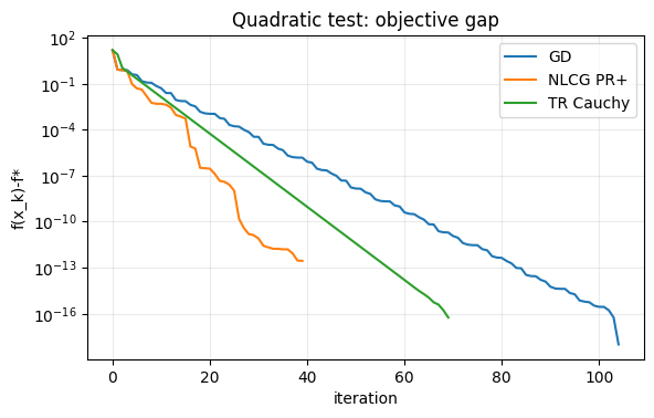
print("GD iterations:", len(h_gd["f"]), "solution:", x_gd)
print("NLCG iterations:", len(h_cg["f"]), "solution:", x_cg)
print("TR-Cauchy iterations:", len(h_tr["f"]), "solution:", x_tr)
GD iterations: 105 solution: [ 0.5075 -1.2239]
NLCG iterations: 40 solution: [ 0.5075 -1.2239]
TR-Cauchy iterations: 70 solution: [ 0.5075 -1.2239]
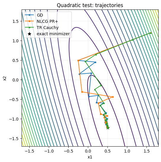
# Trajectories on level sets
grid = np.linspace(-1.7, 1.8, 320)
X, Y = np.meshgrid(grid, grid)
Z = 0.5 * (A[0, 0] * X**2 + 2.0 * A[0, 1] * X * Y + A[1, 1] * Y**2) - b[0] * X - b[1] * Y

P_gd = np.array(h_gd["x"])
P_cg = np.array(h_cg["x"])
P_tr = np.array(h_tr["x"])

fig, ax = plt.subplots(figsize=(6, 6))
ax.contour(X, Y, Z, levels=24, cmap="viridis")
ax.plot(P_gd[:, 0], P_gd[:, 1], "o-", ms=3, lw=1.5, label="GD")
ax.plot(P_cg[:, 0], P_cg[:, 1], "s-", ms=3, lw=1.5, label="NLCG PR+")
ax.plot(P_tr[:, 0], P_tr[:, 1], "^-", ms=3, lw=1.5, label="TR Cauchy")
ax.scatter(x_star_quad[0], x_star_quad[1], c="k", s=60, marker="*", label="exact minimizer")
ax.set_title("Quadratic test: trajectories")
ax.set_xlabel("x1")
ax.set_ylabel("x2")
ax.legend()
ax.set_aspect("equal", "box")
ax.grid(alpha=0.2)
plt.show()
# Convergence histories
fig, ax = plt.subplots(figsize=(6.5, 3.8))
ax.semilogy(np.array(h_gd["f"]) - f_quad(x_star_quad) + 1e-18, label="GD")
ax.semilogy(np.array(h_cg["f"]) - f_quad(x_star_quad) + 1e-18, label="NLCG PR+")
ax.semilogy(np.array(h_tr["f"]) - f_quad(x_star_quad) + 1e-18, label="TR Cauchy")
ax.set_title("Quadratic test: objective gap")
ax.set_xlabel("iteration")
ax.set_ylabel("f(x_k)-f*")
ax.grid(True, which="both", alpha=0.25)
ax.legend()
plt.show()
Test Problem B: Rosenbrock Function
Now use a standard nonconvex benchmark to compare robustness and practical speed:
def f_ros(x):
return 100.0 * (x[1] - x[0]**2)**2 + (1.0 - x[0])**2
def g_ros(x):
return np.array([
-400.0 * x[0] * (x[1] - x[0]**2) - 2.0 * (1.0 - x[0]),
200.0 * (x[1] - x[0]**2),
])
def h_ros(x):
return np.array([
[1200.0 * x[0]**2 - 400.0 * x[1] + 2.0, -400.0 * x[0]],
[-400.0 * x[0], 200.0],
])
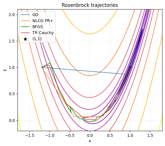
x0 = np.array([-1.2, 1.0])
x_gd_r, h_gd_r = optimize_gd(f_ros, g_ros, x0, maxit=10000, tol=1e-6)
x_cg_r, h_cg_r = optimize_nlcg(f_ros, g_ros, x0, beta_type="PR+", maxit=2000, tol=1e-6, restart_every=25)
x_bfgs_r, h_bfgs_r = optimize_bfgs(f_ros, g_ros, x0, maxit=500, tol=1e-6)
x_tr_r, h_tr_r = optimize_trust_region_cauchy(f_ros, g_ros, h_ros, x0, delta0=0.3, maxit=2000, tol=1e-6)
print("GD iter:", len(h_gd_r["f"]), "x:", x_gd_r, "f:", f_ros(x_gd_r))
print("NLCG iter:", len(h_cg_r["f"]), "x:", x_cg_r, "f:", f_ros(x_cg_r))
print("BFGS iter:", len(h_bfgs_r["f"]), "x:", x_bfgs_r, "f:", f_ros(x_bfgs_r))
print("TR iter:", len(h_tr_r["f"]), "x:", x_tr_r, "f:", f_ros(x_tr_r))
GD iter: 10000 x: [1. 1.] f: 2.7097756887567074e-10
NLCG iter: 780 x: [1. 1.] f: 9.333345059566065e-14
BFGS iter: 35 x: [1. 1.] f: 2.74563522272072e-17
TR iter: 1149 x: [1. 1.] f: 1.174131165677434e-12
# Path plot on Rosenbrock level sets
x1 = np.linspace(-1.8, 1.8, 420)
x2 = np.linspace(-0.2, 2.1, 420)
X1, X2 = np.meshgrid(x1, x2)
Z = 100.0 * (X2 - X1**2)**2 + (1.0 - X1)**2

P_gd = np.array(h_gd_r["x"][::max(1, len(h_gd_r["x"]) // 150)])
P_cg = np.array(h_cg_r["x"][::max(1, len(h_cg_r["x"]) // 150)])
P_bf = np.array(h_bfgs_r["x"])
P_tr = np.array(h_tr_r["x"][::max(1, len(h_tr_r["x"]) // 150)])

fig, ax = plt.subplots(figsize=(6.5, 5.5))
levels = np.logspace(-1, 3, 8)
ax.contour(X1, X2, Z, levels=levels, norm=plt.matplotlib.colors.LogNorm(), cmap="plasma")
ax.plot(P_gd[:, 0], P_gd[:, 1], "-", lw=1.2, label="GD")
ax.plot(P_cg[:, 0], P_cg[:, 1], "-", lw=1.2, label="NLCG PR+")
ax.plot(P_bf[:, 0], P_bf[:, 1], "-", lw=1.6, label="BFGS")
ax.plot(P_tr[:, 0], P_tr[:, 1], "-", lw=1.2, label="TR Cauchy")
ax.scatter([1.0], [1.0], c="k", marker="*", s=70, label="(1,1)")
ax.set_xlim(-1.8, 1.8)
ax.set_ylim(-0.2, 2.1)
ax.set_xlabel("x")
ax.set_ylabel("y")
ax.set_title("Rosenbrock trajectories")
ax.grid(alpha=0.2)
ax.legend(loc="upper left")
plt.show()
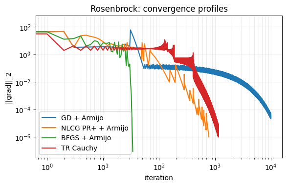
# Gradient norm convergence comparison
fig, ax = plt.subplots(figsize=(6.5, 3.8))
ax.loglog(h_gd_r["gnorm"], label="GD + Armijo")
ax.loglog(h_cg_r["gnorm"], label="NLCG PR+ + Armijo")
ax.loglog(h_bfgs_r["gnorm"], label="BFGS + Armijo")
ax.loglog(h_tr_r["gnorm"], label="TR Cauchy")
ax.set_xlabel("iteration")
ax.set_ylabel("||grad||_2")
ax.set_title("Rosenbrock: convergence profiles")
ax.grid(True, which="both", alpha=0.25)
ax.legend()
plt.show()
Quick Takeaways
GD is robust but can be very slow on narrow valleys.
Nonlinear CG is usually a cheap speed-up over GD.
BFGS gives significantly faster local convergence on smooth problems.
Trust-region globalisation is robust when local models are unreliable.
These are exactly the ingredients we will reuse for reduced PDE-constrained problems.