This notebook illustrates the reduced formulation idea on a tiny linear-quadratic problem.
We consider a constraint (invertible ) and a quadratic objective
Eliminating gives with , hence the reduced cost .
import numpy as np
import matplotlib.pyplot as plt
from pathlib import Path

ROOT = Path.cwd().resolve()
while ROOT != ROOT.parent and not (ROOT / "jupyterbook").exists():
    ROOT = ROOT.parent
OUT_DIR = ROOT / "jupyterbook" / "slides" / "assets"
OUT_DIR.mkdir(parents=True, exist_ok=True)

np.random.seed(0)
Build a Tiny Problem
We’ll work with small matrices and verify that the reduced cost is convex and has a unique minimizer.
n, m = 6, 3
A = np.random.randn(n, n)
A = A.T @ A + 0.5 * np.eye(n)  # SPD => invertible
B = np.random.randn(n, m)
alpha = 1e-2
y_d = np.random.randn(n)

S = np.linalg.solve(A, B)

def J(y, u):
    return 0.5 * np.dot(y - y_d, y - y_d) + 0.5 * alpha * np.dot(u, u)

def f(u):
    y = S @ u
return J(y, u)H = S.T @ S + alpha * np.eye(m)
rhs = S.T @ y_d
u_star = np.linalg.solve(H, rhs)
y_star = S @ u_star
f_star = f(u_star)
f_starnp.float64(0.24237750985949646)A 1D Slice Plot
Plot along a random direction .
d = np.random.randn(m)
d /= np.linalg.norm(d)
t = np.linspace(-2.0, 2.0, 300)
vals = np.array([f(u_star + ti * d) for ti in t])

fig, ax = plt.subplots(figsize=(6.0, 3.5))
ax.plot(t, vals, linewidth=2)
ax.axvline(0.0, linestyle="--", linewidth=1.5)
ax.set_title("Reduced cost along a 1D slice")
ax.set_xlabel("t")
ax.set_ylabel(r"$f(u_* + t d)$")
ax.grid(True, alpha=0.25)
fig.savefig(OUT_DIR / "01_reduced_cost_slice.png", dpi=200, bbox_inches="tight")
# plt.close(fig)

OUT_DIR / "01_reduced_cost_slice.png"
PosixPath('/home/runner/work/nmopt/nmopt/jupyterbook/slides/assets/01_reduced_cost_slice.png')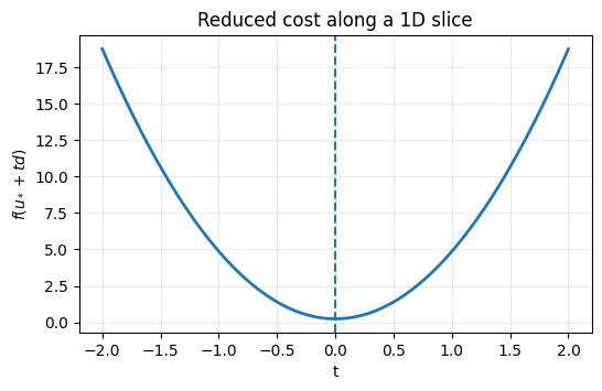
Constrained Minimization Example (2D)
We consider the finite-dimensional constrained problem:
with symmetric positive definite, , .
KKT conditions for the Lagrangian
are
which gives the linear saddle-point system
# 2D constrained minimization: geometry + 1D feasible restriction
A2 = np.array([[3.0, 1.0], [1.0, 2.0]], dtype=float)
B2 = np.array([[1.0, -1.0]], dtype=float)
g2 = np.array([0.5], dtype=float)
kkt = np.block([[A2, -B2.T], [-B2, np.zeros((1, 1))]])
rhs = np.concatenate([np.zeros(2), -g2])
sol = np.linalg.solve(kkt, rhs)
u2_star = sol[:2]
lambda2_star = sol[2]
print('u* =', u2_star)
print('lambda* =', lambda2_star)
# Contours of f(u) and constraint line Bu=g
u1 = np.linspace(-1.2, 1.8, 400)
u2 = np.linspace(-1.2, 1.8, 400)
U1, U2 = np.meshgrid(u1, u2)
F2 = 0.5 * (A2[0, 0] * U1**2 + 2.0 * A2[0, 1] * U1 * U2 + A2[1, 1] * U2**2)
fig, ax = plt.subplots(figsize=(6.2, 4.6))
levels = np.linspace(0.1, 4.0, 9)
ax.contour(U1, U2, F2, levels=levels, cmap='Greens', linewidths=1.5)
line_u1 = np.array([u1.min(), u1.max()])
line_u2 = line_u1 - g2[0] # u2 = u1 - g
ax.plot(line_u1, line_u2, color='purple', linewidth=2.2, label=r'$\varphi(u)=Bu-g=0$')
ax.scatter(u2_star[0], u2_star[1], color='navy', s=50, zorder=5)
ax.text(u2_star[0] + 0.05, u2_star[1] + 0.03, r'$u^\star$', color='navy')
grad_f = A2 @ u2_star
grad_phi = B2.ravel()
scale = 0.28
ax.arrow(u2_star[0], u2_star[1], scale * grad_f[0], scale * grad_f[1],
width=0.004, head_width=0.05, color='tab:red', length_includes_head=True)
ax.text(u2_star[0] + scale * grad_f[0] + 0.03,
u2_star[1] + scale * grad_f[1] + 0.02,
r'$\nabla f(u^\star)$', color='tab:red')
ax.arrow(u2_star[0], u2_star[1], scale * grad_phi[0], scale * grad_phi[1],
width=0.004, head_width=0.05, color='tab:blue', length_includes_head=True)
ax.text(u2_star[0] + scale * grad_phi[0] + 0.03,
u2_star[1] + scale * grad_phi[1] + 0.02,
r'$\nabla \varphi$', color='tab:blue')
ax.set_title('2D constrained minimization: geometry')
ax.set_xlabel(r'$u_1$')
ax.set_ylabel(r'$u_2$')
ax.set_aspect('equal', adjustable='box')
ax.set_xlim(u1.min(), u1.max())
ax.set_ylim(u2.min(), u2.max())
ax.grid(True, alpha=0.25)
ax.legend(loc='upper left')
fig.savefig(OUT_DIR / '01_minimization_geometry.png', dpi=200, bbox_inches='tight')
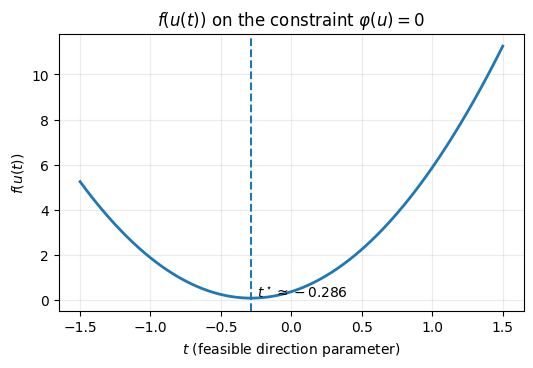
# Restrict to the feasible line u(t)=u0+t d where B d = 0
u0 = np.array([g2[0], 0.0])
d = np.array([1.0, 1.0])
t = np.linspace(-1.5, 1.5, 300)
Uline = u0[None, :] + t[:, None] * d[None, :]
vals_line = 0.5 * np.einsum('bi,ij,bj->b', Uline, A2, Uline)
t_star = t[np.argmin(vals_line)]
fig, ax = plt.subplots(figsize=(6.0, 3.6))
ax.plot(t, vals_line, linewidth=2.0)
ax.axvline(t_star, linestyle='--', linewidth=1.5)
ax.set_title(r'$f(u(t))$ on the constraint $\varphi(u)=0$')
ax.set_xlabel(r'$t$ (feasible direction parameter)')
ax.set_ylabel(r'$f(u(t))$')
ax.grid(True, alpha=0.25)
ax.text(t_star + 0.04, float(np.min(vals_line)) + 0.03, rf'$t^\star \approx {t_star:.3f}$', fontsize=10)
fig.savefig(OUT_DIR / '01_minimization_on_constraint.png', dpi=200, bbox_inches='tight')
OUT_DIR / '01_minimization_geometry.png', OUT_DIR / '01_minimization_on_constraint.png'u* = [ 0.21428571 -0.28571429]
lambda* = 0.3571428571428572
(PosixPath('/home/runner/work/nmopt/nmopt/jupyterbook/slides/assets/01_minimization_geometry.png'),
 PosixPath('/home/runner/work/nmopt/nmopt/jupyterbook/slides/assets/01_minimization_on_constraint.png'))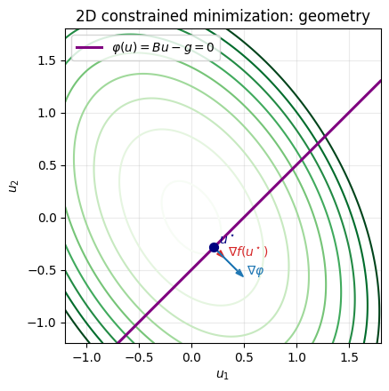
What Changes for PDEs (Hilbert setting)
becomes the solution operator of a PDE (still linear in LQ elliptic problems).
Gradients are computed efficiently via adjoints (no explicit matrix).
The definition of gradients and Hessians passes through the Riesz map, which depends on the choice of inner product in the control space.