|
Fluid structure interaction suite
|


|
|
Fluid structure interaction suite
|
|
Poisson problem, serial version. More...
#include <poisson.h>
Public Member Functions | |
| Poisson () | |
| At construction time, we need to initialize all member functions that are derived from ParameterAcceptor. More... | |
| void | run () |
| Main entry point of the program. More... | |
 Public Member Functions inherited from ParameterAcceptor Public Member Functions inherited from ParameterAcceptor | |
| ParameterAcceptor (const std::string §ion_name="") | |
| unsigned int | get_acceptor_id () const |
| virtual | ~ParameterAcceptor () override |
| virtual void | declare_parameters (ParameterHandler &prm) |
| virtual void | parse_parameters (ParameterHandler &prm) |
| std::string | get_section_name () const |
| std::vector< std::string > | get_section_path () const |
| void | add_parameter (const std::string &entry, ParameterType ¶meter, const std::string &documentation="", ParameterHandler &prm_=prm, const Patterns::PatternBase &pattern=*Patterns::Tools::Convert< ParameterType >::to_pattern()) |
| void | enter_subsection (const std::string &subsection) |
| void | leave_subsection () |
| void | enter_my_subsection (ParameterHandler &prm) |
| void | leave_my_subsection (ParameterHandler &prm) |
| void | serialize (Archive &ar, const unsigned int version) |
| void | subscribe (std::atomic< bool > *const validity, const std::string &identifier="") const |
| void | unsubscribe (std::atomic< bool > *const validity, const std::string &identifier="") const |
| unsigned int | n_subscriptions () const |
| void | list_subscribers (StreamType &stream) const |
| void | list_subscribers () const |
| Public Member Functions inherited from Subscriptor | |
| Subscriptor () | |
| Subscriptor (const Subscriptor &) | |
| Subscriptor (Subscriptor &&) noexcept | |
| virtual | ~Subscriptor () |
| Subscriptor & | operator= (const Subscriptor &) |
| Subscriptor & | operator= (Subscriptor &&) noexcept |
| void | serialize (Archive &ar, const unsigned int version) |
| void | subscribe (std::atomic< bool > *const validity, const std::string &identifier="") const |
| void | unsubscribe (std::atomic< bool > *const validity, const std::string &identifier="") const |
| unsigned int | n_subscriptions () const |
| void | list_subscribers (StreamType &stream) const |
| void | list_subscribers () const |
| void | subscribe (std::atomic< bool > *const validity, const std::string &identifier="") const |
| void | unsubscribe (std::atomic< bool > *const validity, const std::string &identifier="") const |
| unsigned int | n_subscriptions () const |
| void | list_subscribers (StreamType &stream) const |
| void | list_subscribers () const |
Protected Member Functions | |
| void | setup_system () |
| Setup dofs, constraints, and matrices. More... | |
| void | assemble_system () |
| Assemble the matrix and right hand side vector. More... | |
| void | solve () |
| Solve the linear system generated in the assemble_system() function. More... | |
| void | output_results (const unsigned cycle) const |
| Output the solution. More... | |
Protected Attributes | |
| const std::string | component_names = "u" |
| How we identify the component names. More... | |
Grid classes | |
| ParsedTools::GridGenerator< dim, spacedim > | grid_generator |
| A wrapper around GridIn, GridOut, and GridGenerator namespace. More... | |
| ParsedTools::GridRefinement | grid_refinement |
| Grid refinement and error estimation. More... | |
| Triangulation< dim, spacedim > | triangulation |
| The actual triangulation. More... | |
Finite element and dof classes | |
| ParsedTools::FiniteElement< dim, spacedim > | finite_element |
| A wrapper around deal.II FiniteElement classes. More... | |
| DoFHandler< dim, spacedim > | dof_handler |
| The actual DoFHandler class. More... | |
| std::unique_ptr< Mapping< dim, spacedim > > | mapping |
| According to the Triangulation type, we use a MappingFE or a MappingQ, to make sure we can run the program both on a tria/tetra grid and on quad/hex grids. More... | |
Linear algebra classes | |
| AffineConstraints< double > | constraints |
| SparsityPattern | sparsity_pattern |
| SparseMatrix< double > | system_matrix |
| Vector< double > | solution |
| Vector< double > | system_rhs |
| ParsedLAC::InverseOperator | inverse_operator |
| ParsedLAC::AMGPreconditioner | preconditioner |
Forcing terms and boundary conditions | |
| ParsedTools::Constants | constants |
| Constants of the problem. More... | |
| ParsedTools::Function< spacedim > | forcing_term |
| The actual function to use as a forcing term. More... | |
| ParsedTools::Function< spacedim > | exact_solution |
| The actual function to use as a exact solution when computing the errors. More... | |
| ParsedTools::BoundaryConditions< spacedim > | boundary_conditions |
| Boundary conditions used in this class. More... | |
Output and postprocessing | |
| ParsedTools::ConvergenceTable | error_table |
| This is a wrapper around the ParsedConvergenceTable class, that allows you to specify what error to computes, and how to compute them. More... | |
| ParsedTools::DataOut< dim, spacedim > | data_out |
| Wrapper around the DataOut class. More... | |
| unsigned int | console_level = 1 |
| Level of log verbosity. More... | |
| Protected Attributes inherited from ParameterAcceptor | |
| const std::string | section_name |
| std::vector< std::string > | subsections |
Additional Inherited Members | |
| Static Public Member Functions inherited from ParameterAcceptor | |
| static void | initialize (const std::string &filename="", const std::string &output_filename="", const ParameterHandler::OutputStyle output_style_for_output_filename=ParameterHandler::Short, ParameterHandler &prm=ParameterAcceptor::prm, const ParameterHandler::OutputStyle output_style_for_filename=ParameterHandler::DefaultStyle) |
| static void | initialize (std::istream &input_stream, ParameterHandler &prm=ParameterAcceptor::prm) |
| static void | clear () |
| static void | parse_all_parameters (ParameterHandler &prm=ParameterAcceptor::prm) |
| static void | declare_all_parameters (ParameterHandler &prm=ParameterAcceptor::prm) |
| static ::ExceptionBase & | ExcInUse (int arg1, std::string arg2, std::string arg3) |
| static ::ExceptionBase & | ExcNoSubscriber (std::string arg1, std::string arg2) |
| Static Public Member Functions inherited from Subscriptor | |
| static ::ExceptionBase & | ExcInUse (int arg1, std::string arg2, std::string arg3) |
| static ::ExceptionBase & | ExcNoSubscriber (std::string arg1, std::string arg2) |
| Public Attributes inherited from ParameterAcceptor | |
| boost::signals2::signal< void()> | declare_parameters_call_back |
| boost::signals2::signal< void()> | parse_parameters_call_back |
| Static Public Attributes inherited from ParameterAcceptor | |
| static ParameterHandler | prm |
Poisson problem, serial version.
Solve the Poisson equation in arbitrary dimensions and space dimensions. When dim and spacedim are not the same, we solve the Laplace-Beltrami equation. This example is based on the deal.II tutorial step-1, step-2, step-3, step-4, step-5, step-6, and step-38.
The documentation is only a slight rewording of the deal.II tutorials step-3, step-4, step-5, and step-6, where the main differences are related to the classes in the ParsedTools namespace. Basic deal.II classes, like the functions in the GridGenerator namespace, or the FiniteElement class, are replaced with their ParsedTools counterparts, i.e., ParsedTools::GridGenerator, ParsedTools::FiniteElement, ParsedTools::Function, and ParsedTools::DataOut.
In this tutorial program, we solve the Poisson equation:
\[ \begin{cases} - \Delta u = f & \text{ in } \Omega \subset R^{\text{spacedim}}\\ u = u_D & \text{ on } \partial \Omega_D \\ \frac{\partial u}{\partial n} = u_N & \text{ on } \partial \Omega_N \\ \end{cases} \]
We will solve this equation on any grid that can be generated using the ParsedTools::GridGenerator class. An example usage of that class was given in the file MeshHandler.
In this program, the right hand side \(f\), the Dirichlet boundary condition \(u_D\), and the Neumann boundary condition \(u_N\) will be read from a parameter file.
From the basics of the finite element method, we know the steps we need to take to approximate the solution \(u\) by a finite dimensional approximation. Specifically, we first need to derive the weak form of the equation above, which we obtain by multiplying the equation by a test function \(\varphi\) and integrating over the domain \(\Omega\):
\begin{align*} -\int_\Omega \varphi \Delta u = \int_\Omega \varphi f. \end{align*}
This can be integrated by parts:
\begin{align*} \int_\Omega \nabla\varphi \cdot \nabla u -\int_{\partial\Omega} \varphi \mathbf{n}\cdot \nabla u = \int_\Omega \varphi f \end{align*}
The test functions \(\varphi\) are chosen so that they are zero on the Dirichlet part of the boundary \(\gamma_D\), while the Neumann boundary condition is replaced naturally in the integration by parts, and shows up on the right hand side as a boundary supported data. The final weak form reads:
Given \(f (H^1_{0,\Gamma_D} (\Omega))^*\), find \(u \in H^1_{u_D,\Gamma_D} (\Omega)\) such that
\begin{align*} (\nabla\varphi, \nabla u) = (\varphi, f) + \int_{\Gamma_N} u_N \varphi \qquad \forall \varphi \in H^1_{0,\Gamma_D} (\Omega) \end{align*}
In finite elements, we seek an approximation \(u_h(\mathbf x)= U^j \varphi_j(\mathbf x)\) (sum is implied on the repeated indices), where the \(U^j\) are the unknown expansion coefficients we need to determine (the "degrees of freedom" of this problem), and \(\varphi_i(\mathbf x)\) are the finite element shape functions we will use. To define these shape functions, we need the following:
Through these steps, we now have a set of functions \(\varphi_i\), and we can define the weak form of the discrete problem: Find a function \(u_h\), i.e., find the expansion coefficients \(U^j\) mentioned above, so that
\begin{align*} (\nabla\varphi_i, \nabla u_h) = (\varphi_i, f) + \int_{\Gamma_N} u_N \varphi_i, \qquad\qquad i=0\ldots N-1. \end{align*}
This equation can be rewritten as a linear system if you insert the representation \(u_h(\mathbf x)= U^j \varphi_j(\mathbf x)\) and then observe that
\begin{align*} (\nabla\varphi_i, \nabla u_h) &= \left(\nabla\varphi_i, \nabla \Bigl[\sum_j U^j \varphi_j\Bigr]\right) \\ &= \sum_j \left(\nabla\varphi_i, \nabla \left[U^j \varphi_j\right]\right) \\ &= \sum_j \left(\nabla\varphi_i, \nabla \varphi_j \right) U^j. \end{align*}
With this, the problem reads: Find a vector \(U\) so that
\begin{align*} A_{ij} U^j = F_i, \end{align*}
where the matrix \(A\) and the right hand side \(F\) are defined as
\begin{align*} A_{ij} &= (\nabla\varphi_i, \nabla \varphi_j), \\ F_i &= (\varphi_i, f) + \int_{\Gamma_N} u_N \varphi_i. \end{align*}
The final piece of this introduction is to mention that after a linear system is obtained, it is solved using an iterative solver and then postprocessed: we create an output file using the DataOut class that can then be visualized using one of the common visualization programs.
| PDEs::Serial::Poisson< dim, spacedim >::Poisson |
At construction time, we need to initialize all member functions that are derived from ParameterAcceptor.
The general design principle of each of these classes is to take as first argument the name of section where you want store the parameters for the given class, and then the default values that you want to store in the parameter file when you create it the first time.
Definition at line 29 of file poisson.cc.
References triangulation.
| void PDEs::Serial::Poisson< dim, spacedim >::run |
Main entry point of the program.
Just as in all deal.II tutorial programs, the run() function is called from the place where a PDEs::Serial::Poisson object is created, and it is the one that calls all the other functions in their proper order. Encapsulating this operation into the run() function, rather than calling all the other functions from main() of the application makes sure that you can change how the separation of concerns within this class is implemented. For example, if one of the functions becomes too big, you can split it up into two, and the only places you have to be concerned about changing as a consequence are within this very same class, and not anywhere else.
As mentioned above, you will see this general structure – sometimes with variants in spelling of the functions' names, but in essentially this order of separation of functionality – again in all of the following tutorial programs.
Definition at line 250 of file poisson.cc.
References deallog, LogStream::depth_console(), Utilities::int_to_string(), LogStream::pop(), LogStream::push(), and triangulation.
|
protected |
Setup dofs, constraints, and matrices.
This function enumerate all the degrees of freedom and set up matrix and vector objects to hold the system data. Enumerating is done by using DoFHandler::distribute_dofs(), as we have seen in the step-2 example, with the difference that now we pass a ParsedTools::FiniteElement object instead of directly a FiniteElement object.
Definition at line 58 of file poisson.cc.
References AssertThrow, deallog, StandardExceptions::ExcMessage(), get_default_linear_mapping(), DoFTools::make_hanging_node_constraints(), DoFTools::make_sparsity_pattern(), reference_cell(), and triangulation.
|
protected |
Assemble the matrix and right hand side vector.
This function translates the problem in the finite dimensional space to an equivalent linear algebra problmem . These are the main steps that need to be taken into account for this translation:
\begin{align*} A_{ij} &= (\nabla\varphi_i, \nabla \varphi_j) = \sum_{K \in {\mathbb T}} \int_K \nabla\varphi_i \cdot \nabla \varphi_j, \\ F_i &= (\varphi_i, f) = \sum_{K \in {\mathbb T}} \int_K \varphi_i f, \end{align*}
and then approximate each cell's contribution by quadrature:\begin{align*} A^K_{ij} &= \int_K \nabla\varphi_i \cdot \nabla \varphi_j \approx \sum_q \nabla\varphi_i(\mathbf x^K_q) \cdot \nabla \varphi_j(\mathbf x^K_q) w_q^K, \\ F^K_i &= \int_K \varphi_i f + \int_{\Gamma_N} u_N \varphi_i \approx \sum_q \varphi_i(\mathbf x^K_q) f(\mathbf x^K_q) w^K_q + \sum_q \varphi_i(\mathbf x^\Gamma_q) f(\mathbf x^\Gamma_q)w^\Gamma_q, \end{align*}
where \(\mathbb{T} \approx \Omega\) is a Triangulation approximating the domain, \(\mathbf x^K_q\) is the \(q\)th quadrature point on cell \(K\), and \(w^K_q\) the \(q\)th quadrature weight. There are different parts to what is needed in doing this, and we will discuss them in turn next.FEValues really is the central class in the assembly process. One way you can view it is as follows: The FiniteElement and derived classes describe shape functions, i.e., infinite dimensional objects: functions have values at every point. We need this for theoretical reasons because we want to perform our analysis with integrals over functions. However, for a computer, this is a very difficult concept, since they can in general only deal with a finite amount of information, and so we replace integrals by sums over quadrature points that we obtain by mapping (the Mapping object) using points defined on a reference cell (the Quadrature object) onto points on the real cell. In essence, we reduce the problem to one where we only need a finite amount of information, namely shape function values and derivatives, quadrature weights, normal vectors, etc, exclusively at a finite set of points. The FEValues class is the one that brings the three components together and provides this finite set of information on a particular cell \(K\). You will see it in action when we assemble the linear system below.
It is noteworthy that all of this could also be achieved if you simply created these three objects yourself in an application program, and juggled the information yourself. However, this would neither be simpler (the FEValues class provides exactly the kind of information you actually need) nor faster: the FEValues class is highly optimized to only compute on each cell the particular information you need; if anything can be re-used from the previous cell, then it will do so, and there is a lot of code in that class to make sure things are cached wherever this is advantageous.
Definition at line 135 of file poisson.cc.
References deallog, ReferenceCell::get_gauss_type_quadrature(), update_gradients, update_JxW_values, update_quadrature_points, and update_values.
|
protected |
Solve the linear system generated in the assemble_system() function.
After a linear system is obtained, it is solved using an iterative solver. Differently from step-3, we would like to tweak the solver parameters a bit. In order to do so, we use the ParsedLAC::InverseOperator class and the ParsedLAC::AMGPreconditioner, which are wrappers around the deal.II classes that are derived from SolverBase, around the SolverControl class introduced in step-3 (the ParsedLAC::InverseOperator) and around the TrilinosWrappers::PreconditionAMG class, which is compatible also with the deal.II native matrices that we are using here.
The behaviour of the solve function is controlled by the Solver section of the parameter file, i.e.,
Definition at line 201 of file poisson.cc.
References deallog, and inverse_operator().
|
protected |
Output the solution.
When you have computed a solution, you probably want to do something with it. For example, you may want to output it in a format that can be visualized, or you may want to compute quantities you are interested in: say, heat fluxes in a heat exchanger, air friction coefficients of a wing, maximum bridge loads, or simply the value of the numerical solution at a point. This function is therefore the place for postprocessing your solution.
We use the ParsedTools::DataOut class to postprocess our solution. The behaviour of this function is controlled by the section Output of the parameter file :
This wrapper class is a bit more complicated than the one in step-3. Although its usage is very similar, it is important to note that the main difference between ParsedTools::DataOut and DataOut is given by the fact that ParsedTools::DataOut is driven by the parameters above, and simply calls the relevant functions of DataOut with specific arguments, whereas DataOut is usually driven directly by the source code, and requires you to recompile the code if you want, for example, to change the output format, or to disable the writing of high order cells, or to plot also the material ids or the partitioning of the problem.
Definition at line 228 of file poisson.cc.
References deallog, Utilities::int_to_string(), and Utilities::needed_digits().
|
protected |
How we identify the component names.
Many of the classes in the ParsedTools namespace use a string to define their behaviour in terms of the components of a problem. For example, for a scalar problem, one usually needs only to specify the name of the solution with a single component. This is what happens in this program: we use "u" as an identification for the name of the solution, and pass this string around to any class that needs information about components. In general our codes in the FSI-suite will use the functions defined in the ParsedTools::Components namespace to process information about components.
In the scalar case of this program, we have only one component, so this string is not very informative, however, in a more complex case like the PDEs::Serial::Stokes case, we would have spacedim+1 components, spacedim components for the velocity and one component for the pressure. In that case, this string would be "u,u,p" in the two dimensional case, and "u,u,u,p" in the three dimensional case. This string gives information about how we want to group variables, and how we want to treat them in the output as well as how many components our finite element spaces must have.
|
protected |
A wrapper around GridIn, GridOut, and GridGenerator namespace.
The action of this class is driven by the section Grid of the parameter file :
Where you can specify what grid to generate, how to generate it, or what file to read the grid from, and to what file to write the grid to, in addition to the initial refinement of the grid.
|
protected |
Grid refinement and error estimation.
This class is a wrapper around the GridRefinement namespace, and around the KellyErrorEstimator class. The action of this class is governed by the section Grid/Refinement of the parameter file :
where you can specify the number of refinement cycles, the type of error estimator, what marking strategy to use, etc.
At the moment, local refinement is only supported on quad/hex grids. If you try to run the code with a local refinement strategy with a tria/tetra grid, an exception will be thrown at run time.
|
protected |
The actual triangulation.
We allow also for the possibility to use a triangulation that is of co-dimension one or two w.r.t. the space dimension. This is useful when you want to solve Laplace-Beltrami problems, on surfaces, and by the definition of the weak form that we use (which is using the tangent gradient by default), this is what you would get if you use a co-dimension one grid.
|
protected |
A wrapper around deal.II FiniteElement classes.
The action of this class is driven by the parameter Finite element space (u) of the parameter file :
You should make sure that the type of finite element you specify matches the type of triangulation you are using, i.e., FE_Q is supported only on quad/hex grids, while FE_SimplexP is supported only on tri/tetra grids.
The syntax used to specify the finite element type is the same used by the FETools::get_fe_by_name() function.
|
protected |
The actual DoFHandler class.
|
protected |
According to the Triangulation type, we use a MappingFE or a MappingQ, to make sure we can run the program both on a tria/tetra grid and on quad/hex grids.
|
protected |
|
protected |
|
protected |
|
protected |
|
protected |
|
protected |
|
protected |
|
protected |
Constants of the problem.
Most of the problems we will work with, define constants of different types (physical constants, material properties, numerical constants, etc.). The ParsedTools::Constants class allows you to define these in a centralized way, and allows you to share these constants with all the function definitions you may use in your code later on (e.g., the forcing term, or the boundary conditions).
The action of this class is driven by the section Constants of the parameter file :
where you can specify the diffusion coefficient of the problem.
Which constants are defined is built into the ParsedTools::Constants class at construction time (see the source for the constructor Poisson())
|
protected |
The actual function to use as a forcing term.
This is a wrapper around the ParsedFunction class, which allows you to define a function through a symbolic expression (a string) in a parameter file.
The action of this class is driven by the section Functions, with the parameter Forcing term:
You can use any of the numerical constants that are defined in the numbers namespace, such as PI, E, etc, as well as the constants defined at construction time in the ParsedTools::Constants class.
|
protected |
The actual function to use as a exact solution when computing the errors.
This is a wrapper around the ParsedFunction class, which allows you to define a function through a symbolic expression (a string) in a parameter file.
The action of this class is driven by the section Functions, with the parameter Exact solution:
You can use any of the numerical constants that are defined in the numbers namespace, such as PI, E, etc, as well as the constants defined at construction time in the ParsedTools::Constants class.
|
protected |
Boundary conditions used in this class.
The action of this class is driven by the section Boundary conditions of the parameter file :
The way ParsedTools::BoundaryConditions works in the FSI-suite is the following: for every set of boundary ids of the triangulation, you need to specify what boundary conditions are assumed to be imposed on that set. If you only want to specify one type of boundary condition (dirichlet or neumann) on all of the boundary, you can do so by specifying -1 as the boundary id set.
Multiple boundary conditions can be specified, but the same id should should appear only once in the parameter file (i.e., you cannot apply different types of boundary conditions on the same boundary id).
Keep in mind the following caveats:
set Boundary id sets (u) = 0, 1; 2, 3, then boundary ids 0 and 1 will get Neumann boundary conditions, while boundary ids 2 and 3 will get Dirichlet boundary conditions., character, then expression for each component are separated by a semicolumn, and for each boundary id set, are separated by the % character. For example, if you want to specify homogeneous Neumann boundary conditions, and constant Dirichlet boundary conditions you can set the following parameter: set Expressions (u) = 0 % 1.all, a component name, or u.n, or u.t to select normal component, or tangential component in a vector valued problem. For scalar problems, only the name of the component makes sense. This field allows you to control which components the given boundary condition refers to.To summarize, the following is a valid section for the example above:
This would apply Dirichlet boundary conditions on the boundary ids 2 and 3, and homogeneous Neumann boundary conditions on the boundary ids 0 and 1.
|
protected |
This is a wrapper around the ParsedConvergenceTable class, that allows you to specify what error to computes, and how to compute them.
The action of this class is driven by the section Error table of the parameter file :
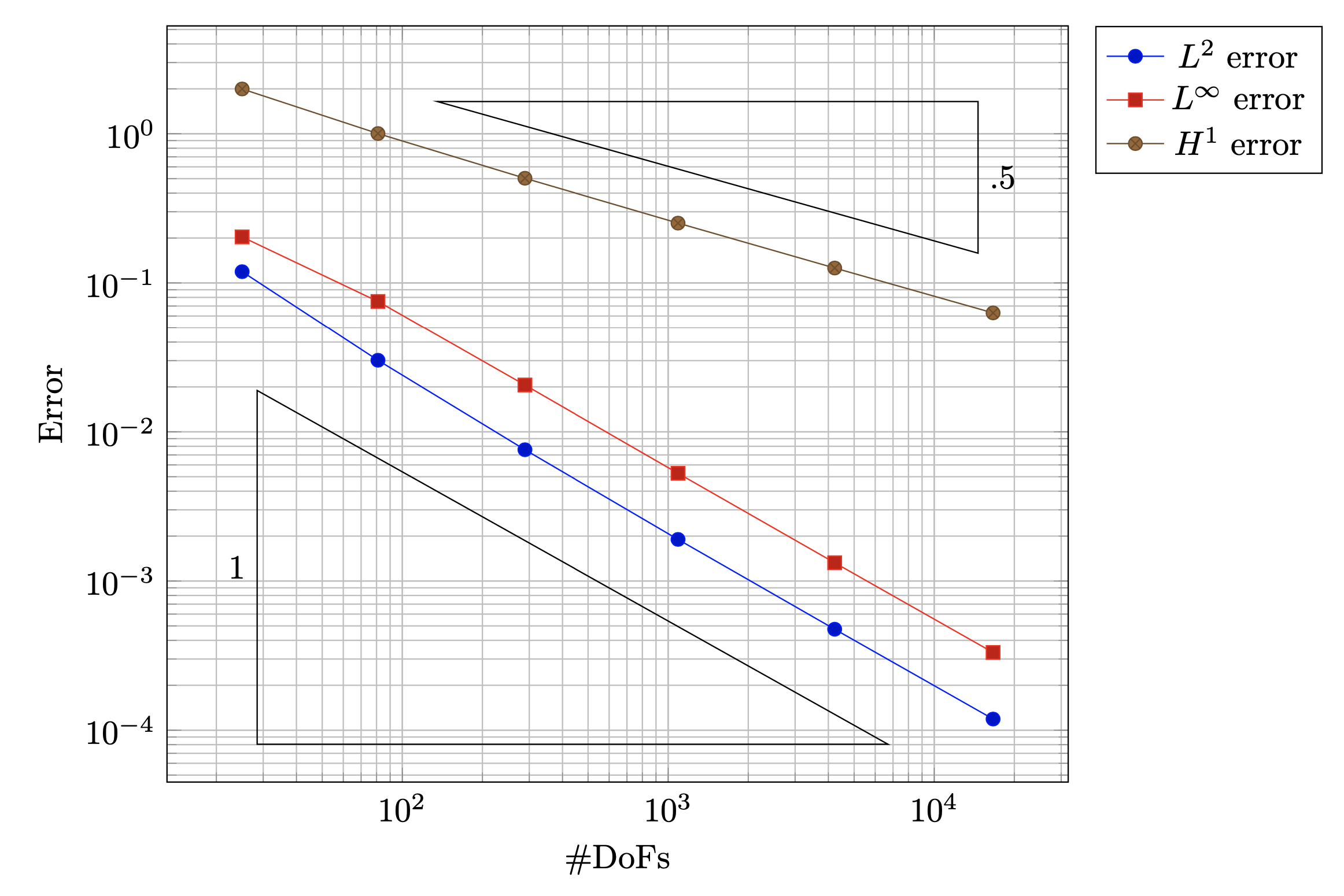
The above code, for example, would produce a convergence table that looks like
The table above can be used as-is to produce high quality pdf outputs of your error convergence rates using the file in the FSI-suite repository latex/quick_convergence_graphs/graph.tex. For example, the above table would result in the following plot:
|
mutableprotected |
Wrapper around the DataOut class.
The action of this class is driven by the section Output of the parameter file :
A similar structure was used in the program dof_plotter.cc.
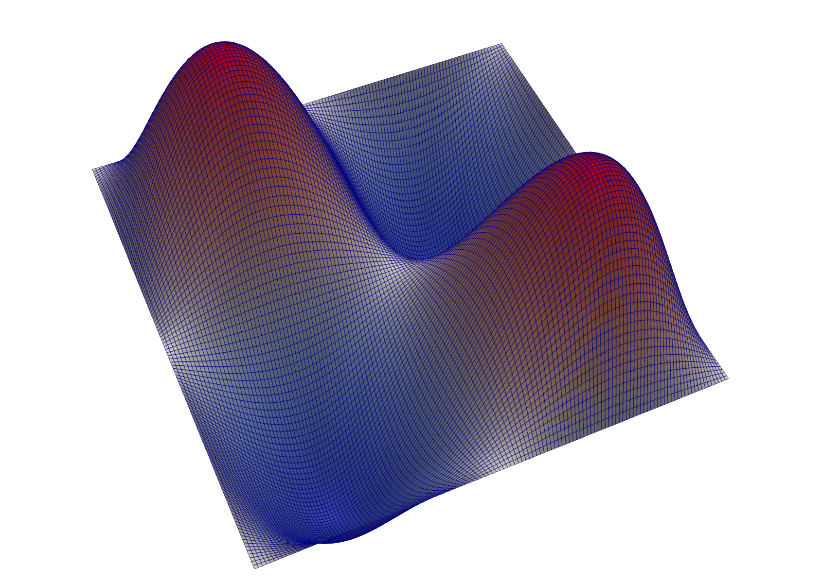
For example, using the configuration specified above, a plot of the solution using the vtu format would look like:
|
protected |
Level of log verbosity.
This is the only "native" parameter of this class. All other parameters are set through the constructors of the classes that inherit from ParameterAcceptor.
The console_level is used to setup the LogStream class, and allows dealii clases to print messages to the console at different level of detail and verbosity.