Overview
This lecture introduces optimal control as an optimization problem constrained by equations. We first build the finite-dimensional analogy, then move to PDE-constrained models.
Logical path of the lecture:
start from a constrained optimization problem in ;
eliminate the state through the model equation when possible;
obtain a reduced optimization problem in the control variable only;
derive first-order conditions in finite dimension;
transfer the same structure to PDE settings.
General Optimal Control Problem
Choose a control variable and a state variable such that
subject to
Key ingredients:
state equation (ODE/PDE/algebraic)
admissible controls
cost functional
optional extra constraints (box constraints, state constraints, etc.)
Forward Problem vs Control Problem
Forward problem:
data are fixed
solve once for
Optimal control:
is unknown
solve the state equation repeatedly inside optimization
Finite-Dimensional Setting (Simultaneous vs Reduced)
Consider
with invertible.
Simultaneous formulation
Optimize in and enforce explicitly.
Interpretation:
optimization variable: the pair ;
coupling: and are linked by the model equation;
computational consequence: every candidate pair must satisfy the constraint.
Reduced formulation
Since is invertible,
where is the control-to-state operator. Then define
and solve
This reduces a finite-dimensional control problem to a standard finite-dimensional optimization problem.
Step-by-step logic:
the constraint defines uniquely as a function of ;
therefore the only independent decision variable is ;
the objective becomes a composite map ;
all constraint information is encoded in .
Existence in Finite Dimensions
A standard existence result for the reduced problem:
If
is lower semicontinuous and bounded from below,
one level set is nonempty, closed, and bounded,
then a minimizer exists.
Reason: in finite dimensions, closed and bounded sets are compact (Weierstrass theorem).
Why this matters for control:
before deriving optimality conditions, we need existence of at least one minimizer;
existence is easy in finite dimension under compactness of level sets;
this argument will fail in infinite dimensions unless additional structure is used.
Unconstrained First/Second-Order Conditions
For convex differentiable on a convex set :
is the first-order optimality condition.
Special case (interior point):
If and is a local minimizer:
is positive semidefinite
If moreover is positive definite, then is a strict local minimizer.
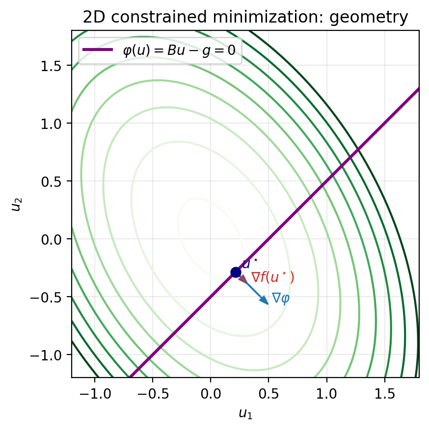
Constrained minimization (2D Example)
Let
with
Logical interpretation:
objective level sets are ellipses (because is SPD);
feasible points lie on an affine line ;
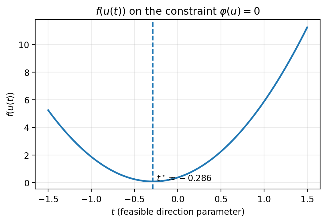
the minimizer is where the first objective level set touches that feasible line.
At an optimal feasible point, is orthogonal to the feasible tangent direction, so it must be parallel to :
Equivalent first-order form:
Meaning:
: feasibility at the solution;
gradient balance: objective gradient is compensated by constraint normal direction;
multiplier : strength/sign of that compensation.
Lagrangian Formalism
Define the Lagrangian
and search for saddle points:
Stationarity gives
For this quadratic/affine case:
which is the KKT linear system
This is the prototype for all later optimality systems:
state/constraint equation;
adjoint or multiplier equation;
coupling through stationarity.
From Finite to Infinite Dimensions
For PDE-constrained control, state/control live in function spaces (typically Hilbert spaces):
state space (e.g. Sobolev spaces)
control space
PDE operator
Typical difficulties:
non-compactness in infinite dimension
weak vs strong convergence issues
differentiability in Banach/Hilbert spaces
adjoint equations for gradient computation
Conceptual continuity with the finite-dimensional case:
same optimization structure;
same reduced-vs-simultaneous viewpoints;
same KKT logic;
only the functional-analytic setting changes.
Prototypical PDE-Constrained Models
Elliptic distributed control
subject to
Parabolic control
with tracking over space-time and Tikhonov regularization.
Flow and inverse problems
Navier-Stokes control (nonlinear constraints)
parameter estimation/data assimilation
Control Constraints
Common box constraints:
They lead to variational inequalities and KKT systems in function spaces.
Typical Variations of OCP Formulations
Many optimal control models keep the same abstract structure but vary in where the control acts, what is observed, and how the objective is measured.
Common variations include:
Localized distributed control: acts only on a subdomain (for example through in the PDE).
Boundary control: appears in Dirichlet/Neumann/Robin boundary conditions on part of .
Initial-condition control: is an unknown initial datum in time-dependent models.
Parameter control: is a coefficient (diffusivity, reaction rate, material parameter), not a source term.
Different tracking norms: replace tracking by , weighted norms, or mixed space-time norms.
Different control penalties: use , , or sparsity-promoting terms (e.g. -type penalties).
Pointwise state constraints: enforce bounds on the state (or output) in the domain or on the boundary.
Multi-objective costs: combine tracking, regularization, and engineering criteria (energy, drag, flux, etc.).
Inverse problems / data assimilation: identify unknown inputs/parameters from measurements with regularization.
Uncertainty-aware OCPs: optimize expected cost, risk measures, or robust worst-case criteria.
These variants motivate why we need a flexible theoretical framework and multiple numerical methods in the rest of the course.
References for This Lecture
F. Tröltzsch, Optimal Control of Partial Differential Equations, Chapter 1
A. Manzoni, A. Quarteroni, S. Salsa, Optimal Control of PDEs, Chapter 1
J. C. De los Reyes, Numerical PDE-Constrained Optimization, Section 1